Download
1 / 22
220 likes | 383 Vues
Computation of Laser Power Output for CW Operation. Konrad Altmann, LAS-CAD GmbH. Pump transition. Laser transition. Energy levels, population numbers, and transitions for a 4-level laser system. Rate Equations for a 4-Level System.

E N D
Computation of Laser Power Output for CW Operation Konrad Altmann, LAS-CAD GmbH
Pump transition Laser transition Energy levels, population numbers, and transitions for a 4-level laser system
Rate Equations for a 4-Level System N(x,y,z) = N2–N1 population inversion density (N1 ~ 0) Rp pump rate W(x,y,z) transition rate due to stimulated emission spontaneous fluorescence life time of upper laser level SL number of laser photons in the cavity mean life time of laser photons in the cavity
The pump rate is given by ηP pump efficiency p0(x,y,z) absorbed pump power density distribution normalized over the crystal volume Sp total number of pump photons absorbed in the crystal per unit of time
The transition rate due to stimulated emission is given by σ stimulated emission cross section n refractive index of laser material s0(x,y,z) normalized distribution of the laser photons
Detailed Rate Equations of a 4-Level Systems Condition for equilibrium
Using the equilibrium conditions, and carrying through some transformations one is getting a recursion relation for the number of laser photons in the cavity This equation can be solved by iterative integration. The integral extends over the volume of the active medium. The iteration converges very fast, as starting condition can be used.
The laser power output is obtained by computing the number of photons passing the output coupler per time unit. This delivers for the power ouput the relation Rout reflectivity of output mirror c vacuum speed of light νL frequency of laser light h Planck's constant optical path length
To compute we divide the time t for one round-trip by the total loss TT during one round-trip Here Lroundtrip represents all losses during one roundtrip additional to the loss at the output coupler. Using the above expression one obtains
Using the above relations one obtains for the laser power output the recursion relation Here is the totally absorbed pump power per time unit, νP is the frequency of the pump light
The next viewgraphs are showing results of com-parison between experimental measurements and simulation for Nd:YAG and Nd:YVO4. The agree-ment between the results turned out to be very good.
Power output vs. pump power for 1.1 at.% Nd:YAG Measurement o—o Computation
Power output vs. pump power for 0.27 at.% Nd:YVO4 Measurement o—o Computation
In similar way the laser power output for a quasi-3-level laser system can be computed Energy levels, population numbers, and transitions for a quasi-3-level laser system
Rate Equations for a Quasi-3-Level System Nt doping density per unit volume
Be transition rate for stimulated emission Batransition rate for reabsorption σe(T(x,y,z)) effective cross section of stimulated emission σa effective cross section of reabsorption c the vacuum speed of light
To solve the rate equation again equilibrium conditions are used
After some transformations this recursion relation is obtained This recursion relation differs from the relation for 4-level-systems only due to the term For the above relation goes over into the relation for 4-level systems
The parameter qσ depends on temperature distribution due to temperature dependence of the cross section σe of stimulated emission. σe can be computed by the use of the method of reciprocity. As shown in the paper of Laura L. DeLoach et al. , IEEE J. of Q. El. 29, 1179 (1993) the following relation can be deducted Zu and Zl are the partition functions of the upper and lower crystal field states EZL is the energy separation between lowest components of the upper and the lower crystal field states. k is Boltzmann's constant T(x,y,z) [K] is the temperature distribution in the crystal as obtained from FEA.
Energy levels and transitions for the • Quasi-3-Level-Material Yb:YAG
Output vs. Input Power for a 5 at. % Yb:YAG Laser Measurements: Laser Group, Univ. Kaiserlautern o o Computation Using Temperature Dep. Stim. Em. Cross Section