Download
1 / 20
230 likes | 341 Vues
Explore how to statistically treat a system in contact with a heat bath and understand the fundamental assumption for isolated systems.

E N D
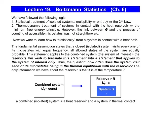
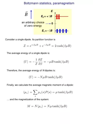
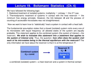
Lecture 19. Boltzmann Statistics (Ch. 6) We have followed the following logic: 1. Statistical treatment of isolated systems: multiplicity entropy the 2nd Law. 2. Thermodynamic treatment of systems in contact with the heat reservoir the minimum free energy principle. However, the link between G and the process of counting of accessible microstates was not straightforward. Now we want to learn how to “statistically” treat a system in contact with a heat bath. The fundamental assumption states that a closed (isolated) system visits every one of its microstates with equal frequency: all allowed states of the system are equally probable. This statement applies to the combined system (the system of interest + the reservoir). We wish to translate this statement into a statement that applies to the system of interest only. Thus, the question: how often does the system visit each of its microstates being in the thermal equilibrium with the reservoir? The only information we have about the reservoir is that it is at the temperature T. Combined system U0 = const Reservoir R U0 - System S a combined (isolated) system = a heat reservoir and a system in thermal contact
The Fundamental Assumption for an Isolated System Isolated the energy is conserved. The ensemble of all equi-energetic states a mirocanonical ensemble i The ergodic hypothesis:an isolated system in thermal equilibrium, evolving in time, will pass through all the accessible microstates states at the same recurrence rate, i.e. all accessible microstates are equally probable. 2 1 The average over long times will equal the average over the ensemble of all equi-energetic microstates: if we take a snapshot of a system with N microstates, we will find the system in any of these microstates with the same probability. Probability of a particular microstate of a microcanonical ensemble = 1 / (# of all accessible microstates) The probability of a certain macrostate is determined by how many microstates correspond to this macrostate – the multiplicity of a given macrostate macrostate Probability of a particular macrostate = ( of a particular macrostate) / (# of all accessible microstates) Note that the assumption that a system is isolated is important. If a system is coupled to a heat reservoir and is able to exchange energy, in order to replace the system’s trajectory by an ensemble, we must determine the relative occurrence of states with different energies.
Reservoir R U0 - System S Systems in Contact with the Reservoir The system – any small macroscopic or microscopic object. If the interactions between the system and the reservoir are weak, we can assume that the spectrum of energy levels of a weakly-interacting system is the same as that for an isolated system. Example: a two-level system in thermal contact with a heat bath. R S 2 1 We ask the following question: under conditions of equilibrium between the system and reservoir, what is the probability P(k) of finding the system S in a particular quantum state kof energy k? We assume weak interaction between R and S so that their energies are additive. The energy conservation in the isolated system “system+reservoir”: U0 = UR+ US = const According to the fundamental assumption of thermodynamics, all the states of the combined (isolated) system “R+S” are equally probable. By specifying the microstate of the system k, we have reduced S to 1 and SS to 0. Thus, the probability of occurrence of a situation where the system is in state kis proportional to the number of states accessible to the reservoirR . The total multiplicity:
SR S(U0) S(U0- 1) S(U0- 2) UR U0 U0- 1 U0- 2 Systems in Contact with the Reservoir (cont.) The ratio of the probability that the systemis in quantum state 1 at energy 1 to the probability that the system is in quantum state 2 at energy 2 is: Let’s now use the fact that S is much smaller than R (US=k << UR). Also, we’ll consider the case of fixed volume and number of particles (the latter limitation will be removed later, when we’ll allow the system to exchange particles with the heat bath (Pr. 6.9 addresses the case when the 2nd is not negligible) 0
Boltzmann Factor T is the characteristic of the heat reservoir exp(- k/kBT) is called the Boltzmann factor This result shows that we do not have to know anything about the reservoir except that it maintains a constant temperature T ! reservoir T The corresponding probability distribution is known as the canonical distribution. An ensemble of identical systems all of which are in contact with the same heat reservoir and distributed over states in accordance with the Boltzmann distribution is called a canonical ensemble. The fundamental assumption for an isolated system has been transformed into the following statement for the system of interest which is in thermal equilibrium with the thermal reservoir: the system visits each microstate with a frequency proportional to the Boltzmann factor. Apparently, this is what the system actually does, but from the macroscopic point of view of thermodynamics, it appears as if the system is trying to minimize its free energy. Or conversely, this is what the system has to do in order to minimize its free energy.
One of the most useful equations in TD+SP... Firstly, notice that only the energy difference = i - j comes into the result so that provided that both energies are measured from the same origin it does not matter what that origin is. Secondly, what matters in determining the ratio of the occupation numbers is the ratio of the energy difference to kBT. Suppose that i = kBT and j = 10kBT . Then (i - j ) /kBT= -9, and The lowest energy level 0 available to a system (e.g., a molecule) is referred to as the “ground state”. If we measure all energies relative to 0 and n0 is the number of molecules in this state, than the number molecules with energy > 0 Problem 6.13. At very high temperature (as in the very early universe), the proton and the neutron can be thought of as two different states of the same particle, called the “nucleon”. Since the neutron’s mass is higher than the proton’s by m = 2.3·10-30 kg, its energy is higher by mc2. What was the ratio of the number of protons to the number of neutrons at T=1011 K?
Problem 6.14. Use Boltzmann factors to derive the exponential formula for the density of an isothermal atmosphere. The system is a single air molecule, with two states: 1 at the sea level (z = 0), 2 – at a height z. The energies of these two states differ only by the potential energy mgz (the temperature T does not vary with z): More problems At home: A system of particles are placed in a uniform field at T=280K. The particle concentrations measured at two points along the field line 3 cm apart differ by a factor of 2. Find the force F acting on the particles. Answer: F = 0.9·10-19 N A mixture of two gases with the molecular masses m1 and m2 (m2 >m1) is placed in a very tall container. The container is in a uniform gravitational field, the acceleration of free fall, g, is given. Near the bottom of the container, the concentrations of these two types of molecules are n1 and n2 respectively (n2 >n1) . Find the height from the bottom where these two concentrations become equal. Answer:
The Partition Function For the absolute values of probability (rather than the ratio of probabilities), we need an explicit formula for the normalizing factor 1/Z: - we will often use this notation The quantity Z, the partition function, can be found from the normalization condition - the total probability to find the system in all allowed quantum states is 1: The Zustandsumme in German or The partition function Z is called “function” because it depends on T, the spectrum (thus, V),etc. Example: a single particle, continuous spectrum. (kBT1)-1 The areas under these curves must be the same (=1). Thus, with increasing T, 1/Z decreases, and Z increases. At T = 0, the system is in its ground state (=0) with the probability =1. T1 < T2 (kBT2)-1 0
Average Values in a Canonical Ensemble We have developed the tools that permit us to calculate the average value of different physical quantities for a canonical ensemble of identical systems. In general, if the systems in an ensemble are distributed over their accessible states in accordance with the distribution P(i), the average value of some quantity x(i) can be found as: In particular, for a canonical ensemble: Let’s apply this result to the average (mean) energy of the systems in a canonical ensemble (the average of the energies of the visited microstates according to the frequency of visits): The average values are additive. The average total energy Utot of N identical systems is: Another useful representation for the average energy (Pr. 6.16): thus, if we know Z=Z(T,V,N), we know the average energy!
Example: energy and heat capacity of a two-level system The partition function: the slope ~ T Ei 2= The average energy: 1= 0 - lnni (check that the same result follows from ) /2 CV The heat capacity at constant volume: 0 T
Partition Function and Helmholtz Free Energy Now we can relate F to Z: Comparing this with the expression for the average energy: This equation provides the connection between the microscopic world which we specified with microstates and the macroscopic world which we described with F. If we know Z=Z(T,V,N),we know everything we want to know about the thermal behavior of a system. We can compute all the thermodynamic properties:
Microcanonical Canonical Our description of the microcanonical and canonical ensembles was based on counting the number of accessible microstates. Let’s compare these two cases: microcanonical ensemble canonical ensemble For a system in thermal contact with reservoir, the partition function Z provides the # of accessible microstates. The constraint: T, V, N – const For a fixed T, the mean energy U is specified, but U can fluctuate. For an isolated system, the multiplicity provides the number of accessible microstates. The constraint in calculating the states: U, V, N – const For a fixed U, the mean temperature T is specified, but T can fluctuate. - the probability of finding a system in one of the accessible states - the probability of finding a system in one of these states - in equilibrium, S reaches a maximum - in equilibrium, F reaches a minimum For the canonical ensemble, the role of Z is similar to that of the multiplicity for the microcanonical ensemble. This equation gives the fundamental relation between statistical mechanics and thermodynamics for given values of T, V, and N, just as S = kBln gives the fundamental relation between statistical mechanics and thermodynamics for given values of U, V, and N.
Boltzmann Statistics: classical (low-density) limit We have developed the formalism for calculating the thermodynamic properties of the systems whose particles can occupy particular quantum states regardless of the other particles (classical systems). In other words, we ignored all kind of interactions between the particles. However, the occupation numbers are not free from the rule of quantum mechanics. In quantum mechanics, even if the particles do not interact through forces, they still might participate in the so-called exchange interaction which is dependent on the spin of interacting particles (this is related to the principle of indistinguishability of elementary particles, we’ll consider bosons and fermions in Lecture 23). This type of interactions becomes important if the particles are in the same quantum state (the same set of quantum numbers), and their wave functions overlap in space: strong exchange interaction weak exchange interaction the average distance btw particles the de Broglie wavelength Boltzmann statistics applies (for N2 molecule, ~ 10-11 m at RT) Violations of the Boltzmann statistics are observed if the the density of particles is very large (neutron stars), or particles are very light (electrons in metals, photons), or they are at very low temperatures (liquid helium), However, in the limit of small density of particles, the distinctions between Boltzmann, Fermi, and Bose-Einstein statistics vanish.
Degenerate Energy Levels If several quantum states of the system (different sets of quantum numbers) correspond to the same energy level, this level is called degenerate. The probability to find the system in one of these degenerate states is the same for all the degenerate states. Thus, the total probability to find the system in a state with energy i is where diis the degree of degeneracy. Taking the degeneracy of energy levels into account, the partition function should be modified: Example: The energy levels of an electron in the hydrogen atom: r where ni = 1,2,... is the principle quantum number (these levels are obtained by solving the Schrödinger equation for the Coulomb potential). In addition to ni, the states of the electron in the H atom are characterized with three other quantum numbers: the orbital quantum number limax = 0,1, ..., ni– 1, the projection of the orbital momentum mli = - li, - li+1,...0, li-1,li, and the projection of spin si= ±1/2. In the absence of the external magnetic field, all electron states with the same ni are degenerate (the property of Coulomb potential). The degree of degeneracy in this case: i di=2ni2 2 d2 =8 1 d1 =2 (for a continuous spectrum, we need another approach)
Problem (final 2005, partition function) • Consider a system of distinguishable particles with five microstates with energies 0, , , , and 2 ( = 1 eV ) in equilibrium with a reservoir at temperature T =0.5 eV. • Find the partition function of the system. • Find the average energy of a particle. • What is the average energy of 10 such particles? the average energy of a single particle: the same result you’d get from this: the average energy of N = 10 such particles:
Consider a system of N particles with only 3 possible energy levels separated by (let the ground state energy be 0). The systemoccupies a fixed volume V and is in thermal equilibrium with a reservoir at temperature T. Ignore interactions between particles and assume that Boltzmann statistics applies. (a) (2) What is the partition function for a single particle in the system? (b) (5) What is the average energy per particle? (c) (5) What is probability that the 2level is occupied in the high temperature limit, kBT >> ? Explain your answer on physical grounds. (d) (5) What is the average energy per particle in the high temperature limit, kBT >> ? (e) (3) At what temperature is the ground state 1.1 times as likely to be occupied as the 2 level? (f) (25) Find the heat capacity of the system, CV, analyze the low-T (kBT<<) and high-T (kBT >> ) limits, and sketch CV as a function of T. Explain your answer on physical grounds. Problem 1 (partition function, average energy) (a) (b) (c) all 3 levels are populated with the same probability (d)
Problem 1 (partition function, average energy) (e) (f) CV Low T (>>): high T (<<): T
H Problem (the average values) A gas is placed in a very tall container at the temperature T. The container is in a uniform gravitational field, the acceleration of free fall, g, is given. Find the average potential energy of the molecules. h # of molecules within dh: 0 For a very tall container (mgH/kBT ):
r 3= -1.5 eV 2= -3.4 eV 1= -13.6 eV Partition Function for a Hydrogen Atom (Pr. 6.9) Any reference energy can be chosen. Let’s choose = 0 in the ground state: 1=0,2=10.2 eV,3=12.1 eV, etc. The partition function: (a) Estimate the partition function for a hydrogen atom at T = 5800K (= 0.5 eV) by taking into account only three lowest energy states. - we can forget about the spin degeneracy – it is the same for all the levels – the only factor that matters is n2 However, if we take into account all discrete levels, the full partition function diverges:
Partition Function for a Hydrogen Atom (cont.) Intuitively, only the lowest levels should matter at >> kBT . To resolve this paradox, let’s go back to our assumptions: we neglected the term PdV in If we keep this term, then For a H atom in its ground state, V~(0.1 nm)3 , and at the atmospheric pressure, PV~ 10-6 eV (negligible correction). However, this volume increases as n3 (the Bohr radius grows as n), and for n=100, PV is already ~1 eV. The PV terms cause the Boltzmann factors to decrease exponentially, and this rehabilitates our physical intuition: the correct partition function will be dominated by just a few lowest energy levels.