A Case Study in Regional Inverse Modeling
200 likes | 346 Vues
A Case Study in Regional Inverse Modeling. Andrew Schuh, Scott Denning, Marek Ulliasz Kathy Corbin, Nick Parazoo. The Question: How is NEE distributed across domain in both time and space. Deterministic Biosphere and Transport Models.

A Case Study in Regional Inverse Modeling
E N D
Presentation Transcript
A Case Study in Regional Inverse Modeling Andrew Schuh, Scott Denning, Marek UlliaszKathy Corbin, Nick Parazoo
The Question:How is NEE distributed across domain in both time and space
Deterministic Biosphere and Transport Models • SiB2.5 is used to predict carbon assimilation and manage energy fluxes at the surface. MODIS fPAR and LAI products are used to drive SiB2.5. • SiB2.5 is coupled to RAMS 5.0 which is used to transport carbon dioxide. Meteorology is forced with Eta 40km reanalysis data • Entire coupled model is run on 150 x 100 40km grid over North America for the time period May 1,2004 through August 31, 2004.
Inversion Methods Available • Bayesian Synthesis Inversion • For many problems the quickest and easiest method • This basic bayesian posterior computation is at core of many inversion methodologies • However, computational concerns arise if the dimensions of the problem get too large
Inversion Methods Available • Kalman filtering techniques • Reduces the effect of the time dimension of inversion problem by putting in state space framework and updating model in time. • EnKF further reduces dimensional constraints by effectively working with a sampled spatial covariance structure. EnKF has also been shown to have some desirable properties for non-linear models.
Inversion Methods Available • What about dealing with the spatial structure of the problem in a hierarchical way? • Inversion can take advantage of implicit spatial structure inherent in many spatial characterizations, like ecoregions • Covariance properties are propagated through a hierarchical covariance structure, independent within levels, thus reducing dimensionality of the covariance
Hierarchical Model (Model Domain) βI=1 βI=2 LEVEL 2 ECOREGIONS LEVEL 3 ECOREGIONS βI=3 βI=4 βI=4,II=1 βI=4,II=2 LEVEL 1 ECOREGIONS βI=4,II=1,III=1 βI=4,II=1,III=2 βI,=4,II=3 βI=4,II=4 βI=4,II=1,III=3 βI=4,II=1,III=4
Example • A backward in time lagrangian particle model (LPDM) was used in conjunction with a 4 month SiB2.5Rams simulation to produce “influence functions” for assimilation and respiration for 34 towers. • Four afternoon observations each day for May 10, 2004 - August 31, 2004 were used at each of the 34 towers.
What about boundary conditions? • Initial SiBRAMS run had constant carbon dioxide for boundary conditions. • What effect might this have on the simulation? • How might corrections be made to these boundary inflow terms?
Boundary conditions • Initial results would seem to imply that boundary conditions can be very important to regional scale inversion using carbon dioxide concentrations • The boundaries also represent a large spatial area, possibly contributing many unknowns to an often already under constrained problem • In order to investigate this component, we begin by investigating the modes of variability in simulated boundary conditions. • Principal Components are generated, using PCTM (N. Parazoo), for May 1, 2003 – August 31, 2003 and May 1,2004 – August 31, 2004. These provide “directions” of maximal variability (in time) in the boundary conditions.
Boundary conditions • The first principal component generally represents about 75% - 85% of the total variation over time with the second representing another 3% - 6%. • The PCs appear to load nicely, particularly zonally. The first principal component is capturing the changing zonal gradient of carbon dioxide while the second appears to capture gradients produced by synoptic activity along the storm track in N.A. • This appears to be a promising dimension reduction of the boundary influence and possibly robust interannually. • An obvious assumption here is that PCTM captures the major modes of variability. Deficiencies in the transport mechanisms of PCTM can not be expected to be captured via these PCs.
Concluding Remarks and future directions • Hierarchical inverse modeling offers many advantages over traditional methods including an implicit spatial correlation structure, multi-scale estimates of variance and computationally efficient covariance characterizations. • Principal components appear to be a promising method of parameterizing uncertainty in the boundary inflow terms • Further directions:- Nesting down to model grid resolution within regions of interest- Investigating real errors in boundary condition estimates- Applying real tower data