Download
1 / 31
330 likes | 544 Vues
13.1 Individual decision making in the face of risk 13.2 Option price and option value 13.3 Risk and irreversibility 13.4 Environmental cost-benefit analysis revisited 13.5 Decision theory: choices under uncertainty 13.6 A safe minimum standard of conservation.

E N D
13.1 Individual decision making in the face of risk 13.2 Option price and option value 13.3 Risk and irreversibility 13.4 Environmental cost-benefit analysis revisited 13.5 Decision theory: choices under uncertainty 13.6 A safe minimum standard of conservation Chapter 13 Irreversibility risk and uncertainty In this chapter you will learn about the difference between risk and uncertainty find out how risk affects environmental decision making and have the concepts of option value and option price explained see how irreversibility affects environmental decision making and learn about quasi-option value consider decision making in the face of uncertainty be introduced to the safe minimum standard and the precautionary principle learn how environmental performance bonds could work
Risk and uncertainty Risk – where all possible consequences of a decision can be completely enumerated and probabilities assigned to each possible ‘state of the world’, ‘state of nature’, ‘state’ Uncertainty – where where all possible consequences of a decision can be enumerated, but probabilities cannot be assigned Radical uncertainty - where all possible consequences of a decision cannot be enumerated Risk/uncertainty distinction not always made in economics Lack of objective probabilities (gambling, insurance) sometimes dealt with by assigning subjective probabilities In many environmental contexts, probabilities are assigned on the basis of modelling – urban air pollution, nuclear accidents The climate change problem exemplifies radical uncertainty
A fair coin will be tossed repeatedly until it lands tail up. If it falls head up at the first toss, the gambler gets £1. If it falls head up at the second toss, the gambler gets £2, at the third toss £4, at the fourth £8, and so on. Tossing continues until the coin falls tail up. How much would somebody be willing to pay for such a gamble? The answer might appear to be ‘an infinite amount’ because the expected monetary value of the gamble is infinite. The expected value is the sum of the probability-weighted possible outcomes, which in this case is the infinite series which has an infinite sum. That anybody would be prepared to pay a very large amount of money for such a gamble violates everyday experience, and the example is known as the Bernoulli, or St Petersburg, paradox. The paradox can be resolved by assuming that individuals assess gambles in terms of expected utility, rather than expected monetary value, and that the utility function exhibits diminishing marginal utility. The relevant outcome is then the infinite series which has a finite sum, so long as there is some upper limit to U, which is what diminishing marginal utility implies. In economics, the basic approach to the analysis of individual behaviour in any kind of risky situation is to assume the maximisation of expected utility and diminishing marginal utility. The St Petersburg paradox
Basic concepts for risk analysis 1 Expected value Expected utility Risk neutrality, aversion, preference Certainty equivalence Cost of risk bearing The expected value of gamble with income outcomes Y1 and Y2 probabilities p1 and p2 is (13.1) The expected utility of the gamble is (13.2) The certainty equivalent of the gamble is the value for Y that solves The cost of risk bearing is the difference between the expected value of the gamble and its certainty equivalent
Basic concepts for risk analysis 2 For U = Ya, 0<a<1, expected utility is (13.3) and the certainty equivalent is the solution for Y in (13.4) Y** is the expected value of the gamble Y* is the certainty equivalent of the gamble For U=Ya, 0<a<1, Y* < Y** This individual is risk averse and CORB = Y** - Y* (13.5) For a = 1, get risk neutrality For risk preference arc ADEB would lie below straight line ACB, with ∂U/∂Y > 0 and ∂2U/∂Y2 > 0
Option price and option value 1 Consider an individual and a national park wilderness area. A – available, the park is open N – the park is closed U(A) –utility for income YA, park open and wants to visit U(N) – utility for income YA, park closed and wants to visit. p1 – probability of N, 1-p1 of A NCA as p1 varies Y** is the expected value of the outcome Y* is the certainty equivalent
Option price and option value 2 YA – Y** is the expected value of the individual’s compensating surplus, E[CS]. YA – Y* is option price, OP, the maximum that the individual would be willing to pay for an option that guaranteed access to an open park. For Figure 13.2 U function, risk aversion, Y** > Y* has OP > E[CS]. OP = E[CS] + OV (13.6) with OV, option value, positive. With risk neutrality, NCA and arc NA coincide and OV would be zero. Option value is a risk aversion premium E[CS] understates the benefit of keeping the park open as risk averse individuals would be willing to pay a premium to avoid risk
Option price and option value 3 Risk also attaches to whether the individual wants to visit The weather determines whether or not the individual wants to visit on a given weekend – fine wants to go, not otherwise. With park open for free WTP for entry on a fine weekend is £10 Probability of fine weather 0.5 E[CS] = £5. Individual told park might be closed next weekend, and offered ticket guaranteeing access. With no risk aversion, ticket is worth E[CS], £5. If the risk averse individual, in order to avoid risk of wanting to go but not being able to get in, is WTP £6 then option price is £6 and option value is £1.
Risk and irreversibility For a risk averse individual, option price exceeds expected compensating surplus by option value. If social decision making adopts consumer sovereignty, given observed actual risk aversion, option price should be used in ECBA. With respect to wilderness development this implies that the level of net development benefits required to justify development needs to be greater than in a world where the future is certain. There are arguments that work in the same direction – require larger net development benefits to justify development – that do not require the risk aversion assumption. These use imperfect knowledge of the future and irreversibility. Wilderness development ( also nuclear power ) can reasonably be regarded as irreversible, given the timescales typically involved in any regeneration. The decision not to develop is reversible.
Identification of maximum net benefit A is flow of wilderness services, decreasing with extent of development. Costs and benefits are functions of A A* - wilderness service flow that corresponds to allocative efficiency A* can be represented as MC(A) = MB(A) Maximum NB(A) MNB(A) = 0
Irreversibility – future known 1 is now. 2 is the future Future net benefits in present value terms Following Krutilla-Fisher arguments, future MNB2 higher than MNB1 for given A Without irreversibility get A2NI > A1NI With irreversibility A2 cannot be larger than A1 Myopia would mean A1NI and A’2 It means period 1 gain abc, period 2 loss edhi. Taking account of irreversibility would mean A1I and A2I – ab = de. Cost of irreversibility in period 1 is abc Cost of irreversibility in period 2 is def
Irreversibility in a risky world At start of period 1 can assign probabilities p to MNB21 and q = (1 – p) to MNB22. Working with the expected value for period 2 leads to A1IR and A2IR Adding risk to irreversibility leads to lower A – more development – than irreversibility alone But, to less development than if irreversibility were ignored.
Quasi-option value 1 Option Period 1 Period 2 Return 1 D D R1 = (Bd1–Cd1) + Bd2 2 P D R2 = Bp1 + (Bd2–Cd2) 3 P P R3 = Bp1 + Bp2 4 D P Is infeasible Where there is the prospect of improved information ‘the expected benefits of an irreversible decision should be adjusted to reflect the loss of options that it entails’ Arrow and Fisher Even if the decision maker is risk-neutral The size of the adjustment is quasi-option value All or nothing development to simplify. Decision to be taken at start of period 1 when period 1 conditions fully known and period 2 outcomes listed and probabilities attached. At the end of period 1, complete knowledge about period 2 will become available The decision at the start of period 1 is whether to permit development Table 13.1 Two – period development/preservation options D – development P – preservation Ri – return to option i Bpt – preservation benefits Bdt – development benefits Cdt – development costs period 2 costs and benefits as present values
Quasi-option value 2 The return to proceeding immediately with development is (13.20) The return to the decision to preserve at the start of period 1 is (13.21) Suppose for moment that decision maker had complete knowledge at start of period 1. Decision would be to develop if Rd>Rp, Rd – Rp>0, which from 13.20 and 13.21 is (13.22) which can be written (13.23) with N1 = (Bd1 – Cd1) – Bp1, that which would actually be known at the start of period 1 The other terms in (13.23) could not be known at the start of period 1, so it is not an operational decision rule. But, by assumption the decision maker does at the start of period 1 know the possible outcomes for Bd2, Bp2 and (Bd2 – Cd2) and can attach probabilities. Question - ? use the rule develop at start of period 1 if (13.24)
Quasi-option value 3 Answer – no, using this rule would ignore the fact that full information will become available at the start of period 2. The decision maker does not have full information at the start of period 1, but she does know the possibilities and probabilities. The proper decision rule is go ahead with development at the start of period 1 if (13.25) Whereas in 13.24 the decision maker uses the maximum of of the expected values of period 2 preservation and development benefits, in 13.25 she uses the expectation of the maximum of period 2 preservation benefits and net development benefits. The left hand side of 13.25 will be larger than the left hand side of 13.24, so the former, ie 13.25, is a harder test to pass at the start of period 1. The difference between the left hand sides of 13.25 and 13.24 is quasi-option value. Quasi-option value is the amount by which a net benefit assessment which simply replaces outcomes by their expectations should be reduced, given irreversibility, to reflect the pay-off to keeping options open by not developing until more information about future conditions is available.
Quasi-option value – a numerical example Two possible period 2 situations, A and B, are differentiated only by what preservation benefits in the future will turnout to be. For A and B, (Bd2 – Cd2) = 6 For A Bp2 = 10, for B Bp2 = 5 pA = pB = 0.5 Then, for 13.24 the third term on the lhs is. For 13.25 we have two possible outcomes Hence so the development gets the go-ahead if (13.26) and following this decision rule, the development gets the go-ahead if (13.27) Suppose N1 + E[Bd2] = 7.75. Then, using 13.24/13.26 development would be decided on at the start of period 1, while using 13.25/13.27 the decision would be to preserve in period 1. The test based on 13.25 is harder to pass than the 13.24-based test. The 13.25 test adds a premium to the 13.24 test – Quasi-option value which is 0.5 here.
Quasi-option value 4 Positive quasi-option value is a general result – Arrow and Fisher 1974 If, as in the numerical example E[Bp2] > E[(Bd2 – Cd2)] then 13.24 becomes (13.28) Now consider max{Bp2, (Bd2 – Cd2)} from 13.26, which is either Bp2 or a larger number.So long as decision maker entertains the possibility that (Bd2 – Cd2) > Bp2, E[max{Bp2, (Bd2 – Cd2)}] will be greater than E[Bp2] and 13.25 which is will be a harder test to pass than 13.28, with where QOV stands for Quasi-option value
Environmental cost-benefit analysis revisited 1 How should ECBA take account of risk? For risk neutrality instead of use (13.29) However, individuals are risk averse and if this is to be reflected in ECBA, it should use (13.30) for the test, where CORBt is the cost of risk bearing at time t. It is sometimes suggested that risk can be dealt with by using expected values and an a higher discount rate: (13.31) where b is the ‘risk premium’. This implies that the cost of risk bearing is decreasing exponentially with time which is not generally the case. CORBt should be estimated over the project lifetime and used as in 13.30.
Environmental cost-benefit analysis revisited 2 Environmental services are typically public goods, so that the risk spreading argument cannot be used to exclude consideration of CORBt. ECBA that does not ignore risk should use either13.30 with E[B(P)]t replaced by E[CS]t and CORBt replaced by OVt, that is (13.32) or replace both E[B(P)]t and CORBt with OPt and use (13.33) where CS is compensating surplus, OV is option value, and OP is option price. Putting numbers to option values and quasi-option values is difficult. Often judgemental allowance is made and sensitivity analysis conducted.
Decision theory: choices under uncertainty 1 C D E A Conserve the wilderness areaas a national park 120 50 10 B Allow the mine to be developed 5 30 140 A game against nature Table 13.2 A pay-off matrix Two strategies A - Preservation B - Development Three states of nature C – High Preservation Benefit Low return to mine D – Intermediate Preservation and development E – Low Preservation Benefit High return to development
Decision theory: choices under uncertainty 2 C C D D E E A Conserve the wilderness areaas a national park A 0 120 0 50 130 10 B 115 20 0 B Allow the mine to be developed 5 30 140 Maximin - select the strategy with the least-bad worst outcome – is A Maximax – select the best of the best outcomes – is B Minimax regret – form the regret matrix with entries that are the difference between the actual pay-off and what it would have been under the best strategy for the given state of nature – minimax on regret by selecting for the lowest of the largest regret - outcome is B Subjective probability assignment – on basis of principle of insufficient reason assign equal probabilities to each outcome and select for largest expected value pay-off – outcome is A for 60 (B is 58.33) Table 13.2 A pay-off matrix Table 13.3 A regret matrix
A safe minimum standard of conservation F U A 130 0 B 0 z Table 13.4 A regret matrix for the possibility of species extinction Radical uncertainty – cannot list all possible outcomes If mine goes ahead, possibly unique, plant population will be destroyed. Project includes attempted re-establishment of plant population at new location. With no previous experience. No way of assigning probability of success to possible prevention of species extinction. F – state of nature favourable, relocation successful U – state of nature unfavourable, relocation unsuccessful A - do not develop B – develop z is an unknown number. Safe minimum standard - use minimax regret assuming z large enough to make A the right strategy. Because species extinction involves an irreversible reduction in the stock of potentially useful resources, of unknown future value. There are two kinds of ignorance Regarding future preferences, needs and technologies About the characteristics of existing species as they relate to future circumstances Presume z is large enough to make A – do not develop – the correct strategy with minimax regret
A modified safe minimum standard SMS is a very conservative rule. Any project that entailed the possibility of species extinction would get stopped. However large, current gains would be foregone for possible avoided future costs, presumed larger. A modified SMS would adopt the strategy that ensures survival of the species provided that it does not entail socially unacceptably large current costs. How to determine what is currently ‘socially unacceptable’? A modified SMS can be applied to target setting for pollution policy – set standards according to efficiency criteria subject to SMS constraints – accord efficiency a lower priority than conservation except where the two conflict, provided that the opportunity costs of conservation are not excessive.
Box 13.1 Stern climate change review 1 Economic activity A schematic representation of the structure of the enhanced greenhouse effect. Dotted lines represent feedback effects. Examples – methane release, weakened carbon sinks. Our knowledge of all of the links is highly imperfect. The climate change problem is characterised by uncertainty Emissions Sinks Concentrations Climate Biosphere Humans Figure 13.6 The enhanced greenhouse effect
Box 13.1 Stern climate change review 2 The 1992 United Nations Framework Convention on Climate Change adopted a Safe Minimum Standard approach to the problem. Article 2, Objectives, states that: The ultimate objective of this Convention and any related legal instruments that the Conference of the Parties may adopt is to achieve, in accordance with the relevant provisions of the Convention, stabilization of greenhouse gas concentrations in the atmosphere at a level that would prevent dangerous anthropogenic interference with the climate system. This is actually a modified SMS in that Article 2 goes on to say that this is subject to enabling 'economic development to proceed in a sustainable manner'. The role of uncertainty is explicitly recognised in Article 3, Principles, where it is stated that 3. The Parties should take precautionary measures to anticipate, prevent or minimize the causes of climate change and mitigate its adverse effects. Where there are threats of serious or irreversible damage, lack of full scientific certainty should not be used as a reason for postponing such measures, ......... The EU also adopts a precautionary approach, and it has operationalised it as meaning that the change in global average temperature should not be more than 2oC above the pre-industrial level. A number of NGOs have endorsed this objective. (It was endorsed at the Copenhagen UNFCC COP December 2009)
Box 13.1 Stern climate change review 3 The review notes the distinction between risk and uncertainty, and that the fact of the latter suggests a precautionary approach to decision making, which is different from risk aversion. In its formal analysis of the costs of climate change the review actually uses the standard expected utility framework with risk aversion. An integrated assessment model, IAM, projects global GDP under business as usual with and without the effects of climate change. The difference gives a trajectory of GDP loss on account of climate change, which is converted to utility and expressed in BGE loss terms as per Box 3.1 here. For each climatic parameter, Stern constructed a subjective probability distribution. For a given scenario IAM run 1000 times with climatic parameters drawn randomly from their distributions. So, for each scenario get 1000 BGE losses, reported as means across 1000 runs together with 5th and 95th percentiles.
Scenario BGE equivalents: % loss in current consumption Climate Economic 5th percentile Mean 95th percentile Baseline Climate Market impacts 0.3 2.1 5.9 Market impacts + risk of catastrophes 0.6 5.0 12.3 Market impacts + risk of catastrophes + non-market impacts 2.2 10.9 27.4 High Climate Market impacts 0.3 2.5 7.5 Market impacts + risk of catastrophes 0.9 6.9 16.5 Market impacts + risk of catastrophes + non-market impacts 2.7 14.4 32.6 Box 13.1 Stern climate change review 4 Table 13.4 Losses on BAU across six scenarios High climate IAM includes feedbacks from methane release and weakened carbon sinks as temperature increases. Utility discount rate 0.01 Elasticity of marginal utility of consumption 1
Box 13.1 Stern climate change review 5 Mitigation costs Bottom-up: 1% of of GDP (range –1 to 3.5%) for cutting to 75% of current level by 2050 – consistent with stabilisation at 550 ppm CO2e. Top-down: 1% of GDP (+/- 3%) for an emissions trajectory leading to stabilisation around 500-550 ppm CO2e. Target setting in terms of concentrations. Stern does not try to optimise. Looks ( chapter 13) at dis-aggregated impacts and costs, and supports with IAM scenario results. ‘the stabilisation goal should lie within the range 450-500 ppm CO2e’ ‘550 ppm CO2e would be a dangerous place to be, with substantial risks of very unpleasant outcome’ aiming below 450 CO2e ‘would impose very high adjustment costs in the near term for relatively small gains, and might not even be feasible’ Stern argument is based a modified safe minimum standard – a target of 550 ppm CO2e is affordable and would avoid the worst that can be envisaged. A target of 450 ppm CO2e would be safer, but would cost a lot more, and may already be infeasible.
The precautionary principle The precautionary principle is closely related to the modified safe minimum standard and is gaining widespread acceptance, at the governmental and intergovernmental levels, as a concept that should inform environmental policy. Statements of the precautionary principle have been made by a number of governments, by individuals, and as part of inter-national agreements. Thus, for example, Principle 15 of the June 1992 Rio Declaration is that: In order to protect the environment, the precautionary approach shall be widely applied by States according to their capabilities. Where there are threats of serious or irreversible damage, lack of full scientific certainty shall not be used as a reason for postponing cost-effective measures to prevent environmental degradation. Like the SMS, the precautionary principle can be taken as saying that there is a presumption against going ahead with projects that have serious irreversible environmental consequences, unless it can be shown that not to go ahead would involve unacceptable costs. The question which arises is whether there are any policy instruments that are consistent with this approach to irreversibility and uncertainty, which could constitute a feasible means for its implementation in such a way as to avoid an outcome that simply prohibits such projects.
Environmental performance bonds 1 Environmental performance bonds have been suggested as a response to the problem of devising a means of project appraisal which takes on board the ideas behind the SMS and the precautionary principle. Some firm which wishes to undertake a project involving major technological innovation, so that there is no past experience according to which probabilities can be assigned to all possible outcomes. In so far as genuine novelty is involved, there is radical uncertainty in that not all of the possible outcomes can be anticipated. An example of such a project would have been the construction of the first nuclear power plant. Assume an environmental protection agency (EPA) without permission from which the firm cannot go ahead with the project. The EPA takes independent expert advice on the project, and comes to a view about the worst conceivable environmental outcome of the project’s going ahead. Approval of the project is then conditional on the firm depositing with the EPA (‘posting’) a bond of $x, where this is the estimate of the social cost of the worst conceivable outcome. The bond is fully or partially returned to the firm at the end of the project’s lifetime (defined by the longest-lasting conceived consequence of the project, not by the date at which it ceases to produce output) according to the damage actually occurring over the lifetime. If there is no damage the firm gets back $x, plus some proportion of the interest. The withheld proportion of the interest is to cover EPA administration costs and to finance EPA research. If the damage actually occurring is $y, the firm gets back $x – $y, with appropriate interest adjustment. For $x equal to or greater than $y, the firm gets nothing back, forfeiting the full value of the bond.
Environmental performance bonds 2 The advantages claimed for such an instrument are in terms of the incentives it creates for the firm to undertake research to investigate environmental impact and means to reduce it, as well as in terms of stopping projects. Suppose that the EPA decides on $x as the size of the bond, and that the firm assesses lifetime project net returns to it as $(x – 1), and accepts that $x is the appropriate estimate of actual damage to arise. Then it will not wish to go ahead with the project. If, however, the firm took the view that actual damage would be $(x – 2) or less, it would wish to go ahead with the project. The firm has, then, an incentive to itself assess the damage that the project could cause, and to research means to reduce that damage. If it does undertake the project it has an ongoing incentive to seek damage-minimising methods of operation, so as to increase the eventual size of the sum returned to it, $x – $y. At the end of the project’s lifetime, the burden of proof as to the magnitude of actual damage would rest with the firm. The presumption would be that the bond was not returnable. It would be up to the firm to convince the EPA that actual damage was less than $x if it wished to get any of its money back. This would generate incentives for the firm to monitor damage in convincing ways, as well as to research means to minimise damage. In the event that damage up to the amount of the bond, $x, occurred, society would have received compensation. If damage in excess of $x had occurred, society would not receive full compensation. $x is to be set at the largest amount of damage seen as conceivable by the EPA at the outset. A socially responsible EPA would take a cautious view of the available evidence, implying a high figure for $x, so that society would not find itself uncompensated.