Tutorial on Risk and Uncertainty
350 likes | 376 Vues
Explore the complexities of risk and uncertainty through Prospect Theory and Expected Utility analysis. Learn about risk aversion, behavioral econometrics, and decision-making applications in various fields.

Tutorial on Risk and Uncertainty
E N D
Presentation Transcript
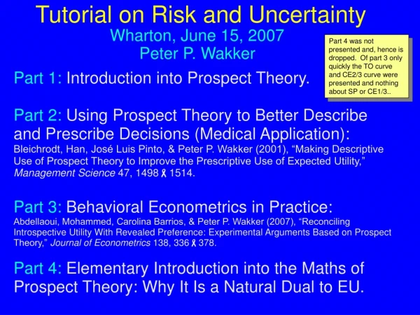
Tutorial on Risk and Uncertainty Wharton, June 15, 2007 Part 4 was not presented and, hence is dropped. Of part 3 only quickly the TO curve and CE2/3 curve were presented and nothing about SP or CE1/3.. Peter P. Wakker Part 1: Introduction into Prospect Theory. Part 2: Using Prospect Theory to Better Describe and Prescribe Decisions (Medical Application): Bleichrodt, Han, José Luis Pinto, & Peter P. Wakker (2001), “Making Descriptive Use of Prospect Theory to Improve the Prescriptive Use of Expected Utility,” Management Science 47, 14981514. Part 3: Behavioral Econometrics in Practice: Abdellaoui, Mohammed, Carolina Barrios, & Peter P. Wakker (2007), “Reconciling Introspective Utility With Revealed Preference: Experimental Arguments Based on Prospect Theory,” Journal of Econometrics 138, 336378. Part 4: Elementary Introduction into the Maths of Prospect Theory: Why It Is a Natural Dual to EU.
p1 p1 x1 x1 . . . . . . . . . . . . xn xn pn pn 2 Part 1: Introduction into Prospect Theory Simplest way to evaluate risky prospects: Expected value p1x1+ ... + pnxn Violated by risk aversion: p1x1+ ... + pnxn
U U concave: p1 x1 x . . . . . . xn pn 3 Bernoulli: Expected utility (EU) p1U(x1) + ... + pnU(xn) Theorem. EU: Risk aversion U concave Measure of risk aversion: –U´´/U´ (Pratt & Arrow). Other often-used index of risk aversion: –xU´´/U´.
4 0.10 0.30 0.50 0.90 0.70 $100 $100 $100 $100 $100 ~ ~ ~ ~ ~ $25 $81 $1 $49 $9 0 0 0 0 0 0.70 0.50 0.10 0.30 0.90 (b) (c) (d) (a) (e) 1 $100 p $ (e) (e) 0.7 $70 (d) (d) (c) (c) (b) 0.3 $30 (b) (a) (a) 0 $0 $0 $100 $30 $70 0 1 0.3 0.7 p $ p. 8 underidentiied next p. Assume following data regarding choice under risk EU: U(9) = 0.30U(100) = 0.30. Psychology since 1950: U(1) = 0.10U(100) + 0.90U(0) = (normalization) 0.10. EU: Psychology: 9 = w(.30)100 Psychology: x = w(p)100. Below is graph of w(p) (= x/100) . EU: U(x) = pU(100) = p. Below is graph of U. 1 = w(.10)100 + w(.90)0 Rotate left and flipped horizontally:
5 Intuitive problem: U reflects value of money;not risk !? U depends on specific nature of money outcome. Different for # hours of listening to music; # years to live; # liters of wine; … nonquantitative outcomes (health states)
6 Lopes (1987, Advances in Experimental ): Risk attitude is more than the psychophysics of money. Empirical problems: Plentiful (Allais, Ellsberg) One more(Rabin 2000): For small amounts EU EV.However, empirically not so!
Psychologists p p x x 0 0 1–p 1–p Joint p x w(p)U(x) 0 1–p p. 4 U/w graph 7 Psychologists: What economists do with money, is better done with probabilities! Economists w increasing, w(0) = 0, w(1) = 1. w(p)x pU(x) At first, for simplicity, we consider U linear. Is proper for moderate amounts of money.
p x y 1–p 8 Data with one nonzero outcome is underidentified for measuring w and U. Fortunately, two-outcome data is sufficiently rich to identify the functions. Then: w(p)U(x) + (1 – w(p))U(y) if x > y 0 if x > 0 > y w(p)U(x) + w–(1–p)U(y)
w inverse-S, (likelihood insensitivity) extreme inverse-S ("fifty-fifty") expected utility motivational pessimism prevailing finding pessimistic "fifty-fifty" cognitive p Abdellaoui (2000); Bleichrodt & Pinto (2000); Gonzalez & Wu 1999; Tversky & Fox, 1997. 9
10 Part 2: Prospect Theory to Better Describe and Prescribe Decisions (Medical Application)
U p Up 11 cure radio- therapy artificial speech recurrency, surgery + cure surgery artificial speech recurrency + nor-mal voice EU normal voice .60 1 .60 0.6 0.4 .744 .144 .9 .16 0.4 0 0 .24 0.6 .744 artificial speech .63 .9 .70 0.7 0.3 .711 .081 .9 .09 0.3 0 0 .21 0.7 .711 Hypothetical standard gamble question: For which p equivalence? Patient with larynx-cancer (stage T3). Radio-therapy or surgery? Patient answers: p = 0.9. Expected utility: U() = 0; U(normal voice) = 1; U(artificial speech) = 0.9 1 + 0.1 0 = 0.9. p artifi-cial speech or 1p Answer: r.th!
Standard gamble question to measure utility: ~ artificial speech U = p EU = p 1 + (1–p) 0 = p Perf. Health 12 p ? 1-p Analysis is based on EU!?!? “Classical Elicitation Assumption” I agree that EU is normative. Tversky, Amos & Daniel Kahneman (1986), “Rational Choice and the Framing of Decisions,” Journal of Business 59, S251S278.P. S251: "Because these rules are normatively essential but descriptively invalid, no theory of choice can be both normatively adequate and descriptively accurate."
13 Tversky, Amos & Daniel Kahneman (1986), “Rational Choice and the Framing of Decisions,” Journal of Business 59, S251S278: “Indeed, incentives sometimes improve the quality of decisions, experienced decision makers often do better than novices, and the forces of arbitrage and competition can nullify some effects of error and illusion. Whether these factors ensure rational choices in any particular situation is an empirical issue, to be settled by observation, not by supposition (p. S273).” Common justification of classical elicitation assumption: EU is normative (von Neumann-Morgenstern). I agree that EU is normative. But not that this would justify SG (= standard gamble = “qol-probability measurement”) -analysis. SG measurement (as commonly done) is descriptive. EU is not descriptive. There are inconsistencies, so, violations. They require correction (? Paternalism!?).
14 Replies to discrepancies normative/descriptive in the literature: (1) Consumer Sovereignty("Humean view of preference"): Never deviate from people's prefs. So, no EU analysis here! However, Raiffa (1961), in reply to violations of EU: "We do not have to teach people what comes naturally.“ We will, therefore, try more. (2)Interact with client (constructive view of preference). If possible, this is best. Usually not feasible (budget, time, capable interviewers …) (3) Measure only riskless utility. However, we want to measure risk attitude! (4) We accept biases and try to make the best of it.
15 That corrections are desirable, has been said many times before. Tversky & Koehler (1994, Psych. Rev.): “The question of how to improve their quality through the design of effective elicitation methods and corrective procedures poses a major challenge to theorists and practitioners alike.” E. Weber (1994, Psych. Bull.) “ …, and finally help to provide more accurate and consistent estimates of subjective probabilities and utilities in situations where all parties agree on the appropriateness of the expected-utility framework as the normative model of choice.” Debiasing (Arkes 1991 Psych. Bull. etc)
16 Schkade (Leeds, SPUDM ’97), on constructive interpretation of preference: “Do more with fewer subjects.” Viscusi (1995, Geneva Insurance): “These results suggest that examination of theoretical characteristics of biases in decisions resulting from irrational choices of various kinds should not be restricted to the theoretical explorations alone. We need to obtain a better sense of the magnitudes of the biases that result from flaws in decision making and to identify which biases appear to have the greatest effect in distorting individual decisions. Assessing the incidence of the market failures resulting from irrational choices under uncertainty will also identify the locus of the market failure and assist in targeting government interventions intended to alleviate these inadequacies.”
17 Million-$ question: Correct how? Which parts of behavior are taken as “bias,” to be corrected for, and which not? Which theory does describe risky choices better? Current state of the art according to me: Prospect theory, Tversky & Kahneman (1992).
1 w+ 1 0 p Figure. The common weighting function (Luce 2000). 18 First deviation from expected utility: probability transformation w- is similar; Second deviation from expected utility: loss aversion/sign dependence. People consider outcomes as gains and losses with respect to their status quo. They then overweight losses by a factor = 2.25.
p PT: U(x) = p + (1-p) 19 EU: U(x) = p. We: is wrong!! Have to correct for above “mistakes.” w+( ) w+( ) w- • Not at all self-evident are: • value/utility of PT = normative utility for EU!? • probability weighting is bias to be corrected for!? • loss aversion is bias to be corrected for!? • Still, these are my beliefs. • Quantitative corrections proposed by • Bleichrodt, Han, José Luis Pinto, & Peter P. Wakker (2001), "Making Descriptive Use of Prospect Theory to Improve the Prescriptive Use of Expected Utility," Management Science 47, 1498–1514.
.00 .01 .02 .03 .04 .05 .06 .07 .08 .09 .0 0.000 0.025 0.038 0.048 0.057 0.064 0.072 0.078 0.085 0.091 .1 0.097 0.102 0.108 0.113 0.118 0.123 0.128 0.133 0.138 0.143 .2 0.148 0.152 0.157 0.162 0.166 0.171 0.176 0.180 0.185 0.189 .3 0.194 0.199 0.203 0.208 0.213 0.217 0.222 0.227 0.231 0.236 .4 0.241 0.246 0.251 0.256 0.261 0.266 0.271 0.276 0.281 0.286 .5 0.292 0.297 0.303 0.308 0.314 0.320 0.325 0.331 0.337 0.343 .6 0.350 0.356 0.363 0.369 0.376 0.383 0.390 0.397 0.405 0.412 .7 0.420 0.428 0.436 0.445 0.454 0.463 0.472 0.481 0.491 0.502 .8 0.512 0.523 0.535 0.547 0.560 0.573 0.587 0.601 0.617 0.633 .9 0.650 0.669 0.689 0.710 0.734 0.760 0.789 0.822 0.861 0.911 20 Standard Gamble Utilities, Corrected through Prospect Theory, for p = .00, ..., .99 E.g., if p = .15 then U = 0.123
21 1 U 0.8 0.6 0.4 0.2 0 0 0.2 0.4 0.6 0.8 1 p Corrected Standard Gamble Utility Curve
*** *** *** ** ** ** * * *** ** * *** *** 0.25 0.20 0.15 0.10 0.05 0.00 0.05 0.10 22 5th 1st 3d 2nd 4th Corrected(Prospect theory) Classical (EU) USG UCE(at 1st = CE(.10), …, at 5th = CE(.90)) USG UTO(at 1st = x1, …, at 5th = x5) UCE UTO(at 1st = x1, …, 5th = x5)
23 Part 3: Behavioral Econometrics in Practice Abdellaoui, Mohammed, Carolina Barrios, & Peter P. Wakker (2007), “Reconciling Introspective Utility With Revealed Preference: Experimental Arguments Based on Prospect Theory,” Journal of Econometrics 138, 336378. 1st utility measurement: Tradeoff (TO) method (Wakker & Deneffe 1996) Completely choice-based.
t1 200,000 ~ _ _ 2/3 2/3 (U(2000)-U(1000)) (U(2000)-U(1000)) ~ 2000 2000 1000 1000 1/3 1/3 ~ = . . . = 26, 1 curve 24 Tradeoff (TO) method (U(t1)-U(t0)) = (U(2000) - U(1000)) U(1000) + U(t1) = U(2000) + U(t0); EU 2000 1000 _ 2/3 U(t1)-U(t0)= (U(2000)-U(1000)) 1/3 6,000 5000 (=t0) = U(t2)-U(t1)= t1 t2 . . . U(t6)-U(t5)= t5 t6
t1 200,000 EU 2000 1000 _ d1 d1 d1 2/3 U(t1)-U(t0)= (U(2000)-U(1000)) ~ 1/3 12,000 5000 (=t0) = ! ? _ _ 2/3 2/3 (U(2000)-U(1000)) (U(2000)-U(1000)) U(t2)-U(t1)= ~ 2000 2000 1000 1000 d2 d2 d2 1/3 1/3 ~ t1 t2 = ? ! . . . . . . = ! ? U(t6)-U(t5)= t5 t6 29, curves; then 31, CE1/3 25 Tradeoff (TO) method Prospect theory: weighted probs (even unknown probs)
1 U 5/6 4/6 3/6 2/6 1/6 0 t3 t4 t5 $ Consequently:U(tj) = j/6. 26 Normalize:U(t0) = 0; U(t6) = 1. t1 t2 t0 t6
Based on direct judgment, not choice-based. 27 2nd utility measurement: Strength of Preference (SP)
28 Strength of Preference (SP) We assume: For which s2 is ? s2 t1 t1t0 U(s2) – U(t1) = U(t1) – U(t0) ~* For which s3 is ? s3 s2 t1t0 U(s3) – U(s2) = U(t1) – U(t0) ~* . . . . . . For which s6 is s6s5 ~* t1t0? U(s6) – U(s5) = U(t1) – U(t0)
CE2/3(PT) SP CE2/3(EU) CE1/3 TO t0= FF5,000 t6= FF26,068 34, which th? PT! (then TO)) 31, CE1/3 33, CE2/3 30, nonTO ,nonEU 32, power? 36,concl 29 7/6 1 U 5/6 4/6 3/6 2/6 1/6 0 FF Utility functions (group averages) TO(PT) = TO(EU) CE1/3(PT) = CE1/3 (EU) (gr.av.) CE2/3(PT) corrects CE2/3 (EU)
30 Question: Could this identity have resulted becausethe TO method does not properly measurechoice-based risky utility? (And, after answering this, what about nonEU?)
For which c2: ? t0 c1 For which c1: ~ ? c2 c2 c3 For which c3: ~ ? t6 29, curves 29, curves 31 3d utility measurement: Certainty equivalent CE1/3 (with good-outcome probability 1/3) EU & RDU & PT (for gr.av.) t0 c2 U(c2) = 1/3 ~ (Chris Starmer, June 24, 2005) on inverse-S: "It is not universal. But if I had to bet, I would bet on this one.". t6 U(c1) = 1/9 U(c3) = 5/9
32 • Questions • Could this identity have resulted because our experiment is noisy(cannot distinguish anything)? • How about violations of EU?
For which d2: ? d1 For which d1: ~ ? d3 For which d3: ~ ? 29, curves 29, curves 33 4th utility measurement: 2/3 Certainty equivalent CE (with good-outcome probability 2/3) CE2/3(EU): CE2/3(PT) (gr.av): t0 d2 U(d2) = 2/3 U(d2) = .51 ~ t6 t0 U(d1) = 4/9 U(d1) = .26 d2 d2 U(d3) = 8/9 U(d3) = .76 t6
34 So, our experiment does have the statistical power to distinguish. And, EU is violated. Which alternative theory to use? Prospect theory.
.51 1/3 2/3 24,TOmethod 35 1 w 1 0 1/3 p Fig.The common probability weighting function. w(1/3) = 1/3; w(2/3) = .51 We re-analyze the preceding measurements(the curves you saw before) in terms of prospect theory; first TO.