Network Layer - an Overview
Network Layer - an Overview. Getting data packets from the source all the way to the destination Dealing with end-to-end transmission Need to know Topology of the communication subnet (routers) Chose paths (routing algorithms). Position of Network Layer. Network Layer Duties. Internetworks.

Network Layer - an Overview
E N D
Presentation Transcript
Network Layer - an Overview • Getting data packets from the source all the way to the destination • Dealing with end-to-end transmission • Need to know • Topology of the communication subnet (routers) • Chose paths (routing algorithms)
Internetworks • Host A -> Host D • 4 LANS, 1 WAN • S1, S2, S3: Switch or Router • f1, f2: Interface • Three links: S1 -> S2 -> s3
Network Layer in an Internetwork Courtesy - From Fig. 19.3 Page 473, Data Communications and Networks, 3rd edition, Forouzan, McGrawHill Prof. Paul Lin
Network Layer at the Source • Creating Source and Destination Address, Fragmentation Courtesy - From Fig. 19.4 Page 473, Data Communications and Networks, 3rd edition, Forouzan, McGrawHill Prof. Paul Lin
Network Layer at Router or Switch • Routing Table, Fragmentation Courtesy - From Fig. 19.5 Page 474, Data Communications and Networks, 3rd edition, Forouzan, McGrawHill Prof. Paul Lin
Network Layer at Destination • Corrupted packet, Fragments Courtesy - From Fig. 196 Page 475, Data Communications and Networks, 3rd edition, Forouzan, McGrawHill Prof. Paul Lin
Figure 24-2 TCP/IP and the OSI Model
Figure 24-3 IP Datagram
INTERNETWORKING PROTOCOL • The internetworking protocol is the transmission mechanism used by TCP/IP Protocol. • It is unreliable and connectionless datagram protocol. • The IP provides no error checking or tracking. • IP assumes the unreliability of the underlying layer and does its best to get a transmission through its destination, but with no guarantee. • IP transports data in Packets called datagrams , each of which transported separately. • Datagrams can travel along different routes and can arrive out of sequence or be duplicated. • IP does not keep track of the routes and has no facility for reordering datagrams once they arrive at their destination.
INTERNETWORKING PROTOCOL • Packets in the IP layer are called datagrams. • A datagram is a variable length packet consisting of two parts: • Header • Data
INTERNETWORKING PROTOCOL • Version: - The first field defines the version number of the IP. (2) Header Length (HLEN): - It defines length of header in a multiple of four bytes. - It varies from 0 to 15. (3) Service Type: - The service type fields defines how the datagram should be handled. - It includes the bit that defines a parity of a datagram. (4) Total Length: - The total length defines the total length of an IP datagram. - It is 2 byte field and can end up to 65,535 bytes.
INTERNETWORKING PROTOCOL (5) Identification: - It is used in fragmentation. - A datagram, when passing through different networks, may be divided into fragments to match the network frame size. - When this happens , each fragment is identified with a sequence number in this field. (6) Flags: - The bit in the flags field deal with fragmentation. (7) Fragmentation offset: - It is a pointer that shows the offset of the data in the original datagram.
INTERNETWORKING PROTOCOL (8) Time to Live: - The time to live field defines the number of hops a datagram can travel before it is discarded. - The source host, when it creates the datagram, sets this field to an initial value. - Then, as datagram travels through the Internet, router by router , each router decrements its value by 1 and if it becomes 0 before it reaches to its final destination, the datagram is discarded. (9) Protocol: - The protocol field defines which upper layer protocol data are encapsulated in the datagram. (TCP, UDP, ICMP, etc.).
INTERNETWORKING PROTOCOL (10) Header Checksum: - This is a 6 bit field used to check the integrity of the header, not the rest of the packet. (11) Source Address: (12) Destination Address: (13) Options: - This field gives more functionality to the IP datagram. - It can carry fields that control routing, timing, management, and alignment.
Routing Algorithms In routing the pathway with the lowest cost is considered the best. Two common methods are used to calculate the shortest path between two routers: (1) Distance Vector Routing (2) Link State Routing
Distance Vector Routing This algorithm works as: Knowledge about the whole network: Each router shares the knowledge about the entire network. It sends all of its collected knowledge about the network to its neighbors. Routing only to neighbors: Each router periodically sends its knowledge about the network only to those routers to which it has direct links. It sends whatever knowledge it has about the whole network through all of its ports. (3) Information sharing at regular intervals: It sends its information at regular interval. for example . After every 30 seconds it sends information.
Distance Vector Routing Table The network ID is the final destination of the packet. The cost is the number of hops a packet must make to get there. Next hop is the router to which a packet must be delivered on its way to particular destination. The table tells a router that it costs x to reach network Y via router Z.
Figure 21-20 Routing Table Distribution
Updating a routing Table When A receives a routing table form B, it uses the information to update it its own table, It says to itself: “ B has sent me a table that shows how its packets can get to network 55 and 14. “ I know that B is my neighbor, so my packets can reach B in one hop.” “ So, if I add one more hop to all of the costs shown in B’s table, the sum will be my cost for reaching those other networks”
Updating a Routing Table rules If the advertised destination is not in the routing table, the router should add the advertised information to the table. If the advertised destination is in the routing table, If the next hop field is the same, the router should replace the entry in the table with the advertised one. Even if the advertised hop count is larger, the advertised entry should replace the entry in the table because the new information invalidated the old. If the next hop field is not the same, If the advertised hop count is smaller than the one in the table, the router should replace the entry in the table with the new one. If the advertised hop count is not smaller, the router should do nothing.
Link State Routing Rules for algorithm: Knowledge about the neighborhood: Instead of sending its entire routing table, a router sends information about its neighborhood only. (2) To all routers: Each router sends this information to every other router on the internetwork, not just to its neighbors. (3) Information sharing when there is a change: Each router sends out information about the neighbors when there is a change.
Packet Cost In distance vector routing , cost refers to a hop count. In link state routing, cost is weighted value based on a variety of factors such as security levels, traffic, or the state of the link.
Different types of address • Three different levels of addresses are used in an internet using TCP/IP protocols: • Physical Address • Logical Address • Port Address
Physical Address • It is also known as link address. • It is defined by its LAN or WAN. • It is lowest level address. • It has an authority over the network. • It can be either • Unicast ( One single recipient) • Multicast (a group of a recipients) • Broadcast ( To be received by all systems in the network.) • Some networks supports all three addresses.
Logical Address • Logical addresses are necessary for universal communication services that are independent of underlying physical networks. • Physical addresses are not adequate in an internetwork environment where different networks can have different address formats. • The logical addresses are designed for internetwork communication. • It is currently 32-bit address that can uniquely define a host connected to the internet. • It can be either unicast, broadcast or multicast.
Port Address • IP address and physical address are necessary for source to destination host transmission. • The aim of internet communication is a process communicating with the another process. • For example, • Computer A can communicate with C by TELNET • Computer A communicate with B by FTP. • For these process occur simultaneously, each process should be labeled. • They are labeled by an address called port address.
Address Space • An address space is the total number of addresses used by the protocol. • If a protocol uses N bits to define an address, the address space is 2n. • IPV4 uses 32-bit address, which means that the address space is of 232 .
Addressing • It can be either • Classful Addressing • Classless Addressing
Addressing • How to define class? For example, 00000001 00001011 00001011 11101111 11000001 10000011 00011011 11111111 10100111 11011011 10001011 01101111 11110011 10011011 11111011 00001111
Class A • Class A is divided into 128 blocks with each block having different netid. • The first block covers addresses from 0.0.0.0 to 0.255.255.255. • The second block covers addresses from 1.0.0.0 to 1.255.255.255 and so on. • Class A addresses were designed for large organizations with large number of hosts or routers attached to that network. • The number of addresses in each block 16,777,216, is larger than the needs of almost organization, so many of them are wasted.