Understanding Non-Linearity in Economic Modeling and its Implications on Optimization
210 likes | 347 Vues
This document explores the concept of non-linearity in economic equations, emphasizing that many economic situations are inherently non-linear despite a reliance on linear approximations. It discusses reasons for non-linearity, local versus global optima in optimization, and introduces quadratic programming as a non-linear problem akin to linear programming. The significance of non-linear models, particularly in portfolio optimization, is examined, highlighting risk-return dynamics and the inherent complexity in analysis. The need for specialized non-linear solutions is stressed, alongside practical modeling tips.

Understanding Non-Linearity in Economic Modeling and its Implications on Optimization
E N D
Presentation Transcript
Roman Keeney AGEC 352 12-03-2012 Non-linearity and Modeling
Introduction • In many situations, economic equations are not linear • We are usually relying on the fact that a linear equation is a good approximation • Even when we assume linearity, sometimes the economics of interest are non-linear • Example: Revenue = Price x Quantity • Quantity = f(Price) • Revenue = Price x f(Price) • dRev/dPrice = Price x df/dPrice + f(Price) • Since this is not a constant, the revenue function when demand depends on price is not constant • Recall our earlier Simon Pies model with the quantity demanded function
Reasons for non-linearity • Non-proportional relationships • Price increases may increase revenue to a point and then decrease it • Depends on demand elasticity at any particular price • Non-additive relationships • E.g. Honey and fruit production • Efficiency of scale • Yield per worker may increase to some point and then decline • Non-linearity of problems results from physical, structural, biological, economic, or logical relationships • Linear models provide good approximations and are MUCH easier to solve
Non-linearity Complications • The degree of non-linearity determines how likely we are to find a solution and have it be the true best choice • Non-linear problems can have local optima • These represent solutions to the problem, but only over a restricted space • Global optima are true best choices, the highest value over the entire feasible set • In LP, any local optima was guaranteed to be a global optima Global Local
Special case of non-linearity: Quadratic Programming • Quadratic programming turns out to be a non-linear problem that is closely related to LP • Quadratic objective equation and linear equality and inequality constraints and non-negativity of variables • The only difference is the functional form (squared terms) of the objective equation • Quadratic function examples • 9X^2 + 4X + 7 • 3X^2 – 4XY + 15Y^2 + 20X - 13Y - 14
QP Example • Min Z = (x – 6)^2 + (y – 8)^2 • s.t. • X <= 7 • Y <= 5 • X + 2Y <=12 • X + Y <= 9 • X, Y >= 0 • Linear constraints, so we could draw them as we always have • Objective equation is quadratic, in fact it is a circle • The 6 and 8 give the coordinates of the center of the circle • Z represents the squared radius of the circle • So, this problem seeks to minimize the squared radius of the circle centered at (6,8) subject to x and y being found in the feasibility set
Example Objective Equation Feasible Space
Spreadsheet modeling • Setup is no different • Need a non-linear formula for the objective • Solver is equipped to solve non-linear problems, just don’t click “assume linear” in the options • Sensitivity • Reduced gradient and Lagrange multiplier replace objective penalties and shadow prices but they are exactly the same • These come from the calculus solution to the problem (Method of Lagrange) • No ranges (allowable increases/decreases)
Why are there differences? • Non-linear functions significantly more complex • Solutions need not occur at corner points of the feasible space • Why is it so useful? • Several models, particularly models involving optimization under risk. • Portfolio model • Minimize the variance of expected returns subject to meeting some minimum expected return
Introduction: Portfolio Model • An individual has 1000 dollars to invest • The 1000 dollars can be allocated a number of ways • Equal split between investments • All in a single investment • Any combination in between • The individual wants to earn high returns • The individual wants low risk
Risk and Returns • Real world investments • Those with high expected returns are those with high risks of losing money • Win big or lose big • Those with low expected returns are those with low risks of losing money • Win small or lose small • Potential losses (downside risk) tend to be larger than upside • Bad outcomes are really bad, Good outcomes are just pretty good
Risks and Returns • Returns are defined by the proportionate gains above the initial investment • Final Amt = (1 + R)* Initial Amt • Risks are defined by the variability (variance) or returns • Given i possible outcomes • Variance is the sum over all i outcomes of • (xi – xmean)^2 • Higher variance means that a given investment produces greater deviations from its average (expected return)
Multiple Objective of Investor • Investors want high returns • Investors want low risk • There are some combined objective equations that look at risk reward tradeoffs but they require knowledge of a decision maker’s risk aversion level • Risk aversion • The concept that people do not like uncertainty about their expected returns/rewards, and in fact will take lower expected returns to avoid some amount of risk/uncertainty when they are making plans or decisions • Absent any knowledge of risk aversion levels we can minimize risk while ensuring a minimum return or maximize return while placing a ceiling on risk
Problem Setup • Two choices • 1) Minimize risk (variance) of the investment strategy • Subject to meeting some minimally acceptable average return for the portfolio • 2) Maximize returns • Subject to not exceeding some maximally acceptable average variance for the portfolio • In practice the second one has become more common • To be a quadratic program, we need to solve option 1 (want the quadratic equation in the objective)
QP Model of Portfolio • Definitions • R1 = returns from investment 1 • Sigma1 = variance of investment 1 • R2 = returns from investment 2 • Sigma2 = variance of investment 2 • Sigma12 = covariance of investments • How much do they vary together? • B = Minimum acceptable return of portfolio • S1 = Maximum share of dollars invested in 1 • S2 = Maximum share of dollars invested in 2
Algebraic Problem • Decision variables X1 and X2 are shares of the total investment • Min Var = X1*X1*sigma1 + X1*X2*sigma12 + X2*X2*sigma2 • Subject to • X1 + X2 = 1 (total investment) • R1*X1 + R2*X2 >= 0.03 (min return) • X1 <= 0.75 (max X1 allocation) • X2 <= 0.90 (max X2 allocation) • Non-negative X1 and X2
Solution • Investment Shares • Inv 1 = 0.36 • Inv 2 = 0.64 • Expected Return • 0.035 • Variance • 0.045 • Sensitivity? • How do investment shares and risk change with changes in minimum expected return
A Different Perspective: Share of X1 and Risk Relative to Mean Return
Results Indicate??? • Risk problems are complex • Investment 1 drives returns up but increases risk • It drives mean returns faster than risk over some range (per last graph) but what is acceptable? • Risk relative to mean is still high for all of these • Only two investments • Adding more choices adds complexity but also adds more ability to mitigate risk • Riskless Assets are often maintained in a portfolio for this reason