Local Linearity
Local Linearity. The idea is that as you zoom in on a graph at a specific point, the graph should eventually look linear. This linear portion approximates the tangent line to the curve at the specific point.

Local Linearity
E N D
Presentation Transcript
Local Linearity • The idea is that as you zoom in on a graph at a specific point, the graph should eventually look linear. • This linear portion approximates the tangent line to the curve at the specific point. • Most of the functions you will encounter are "nearly linear" over very small intervals; that is most functions are locally linear. • All functions that are differentiable at some point where x=c are well-modeled by a unique tangent line in a neighborhood of cand are thus considered locally linear.
A function is differentiable if it has a derivative everywhere in its domain. It must be continuous and smooth. Functions on closed intervals must have one-sided derivatives defined at the end points. p
To be differentiable, a function must be continuous and smooth. Derivatives will fail to exist at: corner cusp discontinuity vertical tangent
Differentiability vs Continuity Theorem: • If f is differentiable at a, then f is continuous at a. • *The converse to this theorem is false. • A continuous function is not necessarily differentiable.
The derivative is the slope of the original function. The derivative is defined at the end points of a function on a closed interval.
Warning: The calculator may return an incorrect value if you evaluate a derivative at a point where the function is not differentiable. Examples: nDeriv(1/x,x,0) returns 1000000 on a TI-84, but -∞on a TI-89 nDeriv(abs(x),x,0) returns 0 on a TI-84, but +/-1 on a TI-89
Graphers calculate numerical derivatives by using difference quotients (the same way you’ve been doing it). Forward difference quotient: Backward difference quotient: Symmetric difference quotient:
If a and b are any two points in an interval on which f is differentiable, then takes on every value between and . Between a and b, must take on every value between and . Intermediate Value Theorem for Derivatives p
Given f(x) = 2x3–3x2 – 6x+2 • Plot the derivative • What type of function is the derivative? • Quadratic (one degree less than f(x)) • When the derivative is 0, what is happening to the graph of the function? • There is either a local max or local min • At x = -1 (local max: f(x) changes from increasing to decreasing) • At x = 2 (local min : f(x) changes from decreasing to increasing)
Let g(x) = f(x) + 5 • Graph in Y3 • Graph the derivative of g in Y4 • How does the derivative of f compare to the derivative of g? • The derivative is the same. The vertical shift does not alter the rate of change. Thus, the derivative remains the same.
Increasing/Decreasing Test • If f '(x) is > 0 on an interval, then f is increasing on that interval. • If f '(x) is < 0 on an interval, then f is decreasing on that interval.
Suppose that c is a critical number of a continuous function f: • If f ' changes from positive to negative at c, then f has a local maximum at c. • If f ' changes from negative to positive at c, then f has a local minimum at c. • (x = c is a critical number of the function f(x) if f ' (c) = 0 or f ' (c) does not exist.