Download
1 / 44
440 likes | 582 Vues
Lecture 4: Informed Heuristic Search. ICS 270a Winter 2003. Summary. Heuristics and Optimal search strategies heuristics hill-climbing algorithms Best-First search A*: optimal search using heuristics Properties of A* admissibility, monotonicity, accuracy and dominance efficiency of A*

E N D
Lecture 4: Informed Heuristic Search ICS 270a Winter 2003
Summary • Heuristics and Optimal search strategies • heuristics • hill-climbing algorithms • Best-First search • A*: optimal search using heuristics • Properties of A* • admissibility, • monotonicity, • accuracy and dominance • efficiency of A* • Branch and Bound • Iterative deepening A* • Automatic generation of heuristics
Problem: finding a Minimum Cost Path • Previously we wanted an arbitrary path to a goal. • Now, we want the minimum cost path to a goal G • Cost of a path = sum of individual transitions along path • Examples of path-cost: • Navigation • path-cost = distance to node in miles • minimum => minimum time, least fuel • VLSI Design • path-cost = length of wires between chips • minimum => least clock/signal delay • 8-Puzzle • path-cost = number of pieces moved • minimum => least time to solve the puzzle
Heuristic functions • 8-puzzle • W(n): number of misplaced tiles • Manhatten distance • Gaschnig’s • 8-queen • Number of future feasible slots • Min number of feasible slots in a row • Travelling salesperson • Minimum spanning tree • Minimum assignment problem
Best first (Greedy) search: f^(n) = number of misplaced tiles
Hill climbing, Greedy search • Example: • 8-queen, traveling salesperson, 8-puzzle, finding routes • Not systematic, • based on local optimization, memoryless, used by humans • Uses an evaluation heuristic function • that evaluates how far we are from the goal • Very greedy: • Expand current node and select the best among its children only if it is better than its own value until found a solution or reached a plateau. Keep only current node. • Greedy: • Expand current node and select the best among its children. Keep current path
Problems with Greedy Search • Not complete • Get stuck on local minimas and plateaus, • Irrevocable, • Infinite loops • Can we incorporate heuristics in systematic search?
Informed search - Heuristic search • How to use heuristic knowledge in systematic search? • Where ? (in node expansion? hill-climbing ?) • Best-first: • select the best from all the nodes encountered so in OPEN. • “good” use heuristics • Heuristic estimates value of a node • promise of a node • difficulty of solving the subproblem • quality of solution represented by node • the amount of information gained. • f(n)- heuristic evaluation function. • depends on n, goal, search so far, domain
Best-First Algorithm BF (*) 1. Put the start node s on a list called OPEN of unexpanded nodes. 2. If OPEN is empty exit with failure; no solutions exists. 3. Remove the first OPEN node n at which f is minimum (break ties arbitrarily), and place it on a list called CLOSED to be used for expanded nodes. 4. Expand node n, generating all it’s successors with pointers back to n. 5. If any of n’s successors is a goal node, exit successfully with the solution obtained by tracing the path along the pointers from the goal back to s. 6. For every successor n’ on n:a. Calculate f (n’).b. if n’ was neither on OPEN nor on CLOSED, add it to OPEN. Attach a pointer from n’ back to n. Assign the newly computed f(n’) to node n’.c. if n’ already resided on OPEN or CLOSED, compare the newly computed f(n’) with the value previously assigned to n’. If the old value is lower, discard the newly generated node. If the new value is lower, substitute it for the old (n’ now points back to n instead of to its previous predecessor). If the matching node n’ resided on CLOSED, move it back to OPEN. • Go to step 2. * With tests for duplicate nodes.
A*- a special Best-first search • Goal: find a minimum sum-cost path • Notation: • c(n,n’) - cost of arc (n,n’) • g^(n) = cost of current path from start to node n in the search tree. • h^(n) = estimate of the cheapest cost of a path from n to a goal. • Special evaluation function: f = g+h • f(n) estimates the cheapest cost solution path that goes through n. • h(n) is the true cheapest cost from n to a goal. • g(n) is the true shortest path from the start s, to n. • If the heuristic function, h^, always underestimate the true cost (h^(n) is smaller than h(n)), then A* is guaranteed to find an optimal solution.
The Road-Map • Find shortest path between city A and B
B C A 10.4 6.7 4.0 11.0 G S 8.9 3.0 6.9 D F E 4 1 B C A 2 5 G 2 S 3 5 4 2 D F E
Example of A* Algorithm in action S 5 + 8.9 = 13.9 2 +10.4 = 12..4 D A 3 + 6.7 = 9.7 D B 4 + 8.9 = 12.9 7 + 4 = 11 8 + 6.9 = 14.9 6 + 6.9 = 12.9 E C E Dead End F B 10 + 3.0 = 13 11 + 6.7 = 17.7 G 13 + 0 = 13
Algorithm A* (with any h on search Graph) • Input: a search graph problem with cost on the arcs • Output: the minimal cost path from start node to a goal node. • 1. Put the start node s on OPEN. • 2. If OPEN is empty, exit with failure • 3. Remove from OPEN and place on CLOSED a node n having minimum f. • 4. If n is a goal node exit successfully with a solution path obtained by tracing back the pointers from n to s. • 5. Otherwise, expand n generating its children and directing pointers from each child node to n. • For every child node n’ do • evaluate h(n’) and compute f(n’) = g(n’) +h(n’)= g(n)+c(n,n’)+h(n) • If n’ is already on OPEN or CLOSED compare its new f with the old f and attach the lowest f to n’. • put n’ with its f value in the right order in OPEN • 6. Go to step 2.
Behavior of A* - Termination • The heuristic function h(n) is called admissible if h(n) is never larger than h*(n), namely h(n) is always less or equal to true cheapest cost from n to the goal. • A* is admissible if it uses an admissible heuristic, and h(goal) = 0. • Theorem (completeness) (Hart, Nillson and Raphael, 1968) • A* always terminates with a solution path if • costs on arcs are positive, above epsilon • branching degree is finite. • Proof: The evaluation function f of nodes expanded must increase eventually until all the nodes on an optimal path are expanded .
Behavior of A* - Completeness • Theorem (completeness for optimal solution) (HNL, 1968): • If the heuristic function is admissible than A* finds an optimal solution. • Proof: • 1. A* will expand only nodes whose f-values are less (or equal) to the optimal cost path C* (f(n) less-or-equal c*). • 2. The evaluation function of a goal node along an optimal path equals C*. • Lemma: • Anytime before A* terminates there exists and OPEN node n’ on an optimal path with f(n’) <= C*.
Consistent (Monotone) heuristics • If in the search graph the heuristic function satisfies triangle inequality for every n and its child node n’: h^(ni) less or equal h^(nj) + c(ni,nj) • when h is monotone, the f values of nodes expanded by A* are never decreasing. • When A* selected n for expansion it already found the shortest path to it. • When h is monotone every node is expanded once (if check for duplicates). • Normally the heuristics we encounter are monotone • the number of misplaced ties • Manhattan distance • air-line distance
Dominance and pruning power of heuristics • Definition: • A heuristic function h dominates h’ (more informed than h) if both are admissible and for every node n, h(n) is greater than h’(n). • Theorem (Hart, Nillson and Raphale, 1968): • An A* search with a dominating heuristic function h has the property that any node it expands is also expanded by A* with h’. • Question: Is manhattan distance more informed than the number of misplaced tiles? • Extreme cases • h = 0 • h = h*
Complexity of A* • A* is optimally efficient (Dechter and Pearl 1985): • It can be shown that all algorithms that do not expand a node which A* did expand (inside the contours) may miss an optimal solution • A* worst-case time complexity: • is exponential unless the heuristic function is very accurate • If h is exact (h = h*) • search focus only on optimal paths • Main problem: space complexity is exponential • Effective branching factor: • logarithm of base (d+1) of average number of nodes expanded.
Additional properties • A* expands every path along which f^(n) < C* • A* will never expand any node s.t f^(n) > C* • If h is monotone A* will expand any node such that f^(n) <C* • Therefore A* expands all the nodes for which f^(n) < C* and a subset of the nodes for which f^(n) = C*. • Therefore if h1(n) < h2(n) clearly the subset of nodes expanded is smaller.
Effectiveness of A* Search Algorithm Average number of nodes expanded d IDS A*(h1) A*(h2) 2 10 6 6 4 112 13 12 8 6384 39 25 12 364404 227 73 14 3473941 539 113 20 ------------ 7276 676 Average over 100 randomly generated 8-puzzle problems h1 = number of tiles in the wrong position h2 = sum of Manhattan distances
Pseudocode for Branch and Bound Search(An informed depth-first search) Initialize: Let Q = {S} While Q is not empty pull Q1, the first element in Q if Q1 is a goal compute the cost of the solution and update L <-- minimum between new cost and old cost else child_nodes = expand(Q1), <eliminate child_nodes which represent simple loops>, For each child node n do: evaluate f(n). If f(n) is greater than L discard n. end-for Put remaining child_nodes on top of queue in the order of their evaluation function, f. end Continue
B C A 10.4 6.7 4.0 11.0 G S 8.9 3.0 6.9 D F E 4 1 B C A 2 5 G 2 S 3 5 4 2 D F E
Example of Branch and Bound in action S 2 5 D A
Properties of Branch-and-Bound • Not guaranteed to terminate unless has depth-bound • Optimal: • finds an optimal solution • Time complexity: exponential • Space complexity: linear
Iterative Deepening A* (IDA*)(combining Branch-and-Bound and A*) • Initialize: f <-- the evaluation function of the start node • until goal node is found • Loop: • Do Branch-and-bound with upper-bound L equal current evaluation function • Increment evaluation function to next contour level • end • continue • Properties: • Guarantee to find an optimal solution • time: exponential, like A* • space: linear, like B&B.
Inventing Heuristics automatically • Examples of Heuristic Functions for A* • the 8-puzzle problem • the number of tiles in the wrong position • is this admissible? • the sum of distances of the tiles from their goal positions, where distance is counted as the sum of vertical and horizontal tile displacements (“Manhattan distance”) • is this admissible? • How can we invent admissible heuristics in general? • look at “relaxed” problem where constraints are removed • e.g.., we can move in straight lines between cities • e.g.., we can move tiles independently of each other
Inventing Heuristics Automatically (continued) • How did we • find h1 and h2 for the 8-puzzle? • verify admissibility? • prove that air-distance is admissible? MST admissible? • Hypothetical answer: • Heuristic are generated from relaxed problems • Hypothesis: relaxed problems are easier to solve • In relaxed models the search space has more operators, or more directed arcs • Example: 8 puzzle: • A tile can be moved from A to B if A is adjacent to B and B is clear • We can generate relaxed problems by removing one or more of the conditions • A tile can be moved from A to B if A is adjacent to B • ...if B is blank • A tile can be moved from A to B.
Generating heuristics (continued) • Example: TSP • Finr a tour. A tour is: • 1. A graph • 2. Connected • 3. Each node has degree 2. • Eliminating 2 yields MST.
Automating Heuristic generation • Use Strips representation: • Operators: • Pre-conditions, add-list, delete list • 8-puzzle example: • On(x,y), clear(y) adj(y,z) ,tiles x1,…,x8 • States: conjunction of predicates: • On(x1,c1),on(x2,c2)….on(x8,c8),clear(c9) • Move(x,c1,c2) (move tile x from location c1 to location c2) • Pre-cond: on(x1.c1), clear(c2), adj(c1,c2) • Add-list: on(x1,c2), clear(c1) • Delete-list: on(x1,c1), clear(c2) • Relaxation: • 1. Remove from prec-dond: clear(c2), adj(c2,c3) #misplaced tiles • 2. Remove clear(c2) manhatten distance • 3. Remove adj(c2,c3) h3, a new procedure that transfer to the empty location a tile appearing there in the goal
Heuristic generation • The space of relaxations can be enriched by predicate refinements • Adj(y,z) iff neigbour(y,z) and same-line(y,z) • The main question: how to recognize a relaxed problem which is easy. • A proposal: • A problem is easy if it can be solved optimally by agreedy algorithm • Heuristics that are generated from relaxed models are monotone. • Proof: h is true shortest path I relaxed model • H(n) <=c’(n,n’)+h(n’) • C’(n,n’) <=c(n,n’) • h(n) <= c(n,n’)+h(n’) • Problem: not every relaxed problem is easy, often, a simpler problem which is more constrained will provide a good upper-bound.
Improving Heuristics • If we have several heuristics which are non dominating we can select the max value. • Reinforcement learning.
Planning, Acting and Learning(Nillson Ch 10) • Sense/Plan/Act cycle: • Uncertainty in sensors of the environment • Effect of action uncertain • Dynamic world is changing in an unpredictable manner • Agent may need to plan quickly before plan is complete • Computational resources for computing a complete plan are insufficient. • Approaches • Markov decision processes (MDPs) \ • Partially observable Markov Decision Processes (POMDPs) • Sense/Plan/Act architecture: execute first action and replan • Algorithms: • Aaproximate search • Island driven search and hierarchical search • Limited Horizon search • Learning Heuristic functions (during simulation or execution) • Reinforcement learning
Limited Horizon Search • When search to completion is too costly. Given a time limit select an action. • Search to a predefined horizon of depth d. • We want to find an optimal path to a node at depth d whose evaluation function is smallest. • Take first action to n*, sense the resulting state and iterate by searching again. • Use Branch and Bound with the evaluation function f(n) (the bound is called alpha-cutoff, analogous to alpha-beta in games). • Special case , d=1, leads to greedy search:
Learning Heuristic FunctionsLearning Real time A* (LRTA*) • If there is no good heuristic and the explicit graph can remembered. • When a good model is available, learning can be done during simulation • Otherwise, learning can be done during actual execution • Learning with a good model • Initialize h^=0 for every node • After expanding a child node or ni update: • h^ can be stored in a table. • h(goal)=0 • A* will be not better than uniform cost after first time to a goal
Learning Heuristic functionsReinforcement learning (Sutton 1990) • When the agent does not have a model he can use the same update rule during execution, does random walk initially until a goal is reached. • The effect of actions are learnt during execution. Learn explicit graph. • A visited state is recorded and its h is updated: • Initially h^(n) = 0. • Action: choose next action a s.t. • Keep truck of all nodes • Problems: Learning suboptimal path • Remedied: allow occasional random actions.
Learning an implicit heuristic during execution • When storing all nodes is NOT practical • Guess a set of relevant features f a state • (P(n): Manhattan distance, W(n), number of misplaced tiles.) • Assume a linear weighted function. • Start with arbitrary weights. When stumble on a goal update the weights minimizing sum square errors when all the instances on the paths are examples. The process is performed iteratively over several searches. • Temporal difference(Sutton 1988): after expanding node ni to produce successor nodes nj we adjust the weight so that:
Summary • In practice we often want the goal with the minimum cost path • Exhaustive search is impractical except on small problems • Heuristic estimates of the path cost from a node to the goal can be efficient in reducing the search space. • The A* algorithm combines all of these ideas with admissible heuristics (which underestimate) , guaranteeing optimality. • Properties of heuristics: • admissibility, monotonicity, dominance, accuracy • Branch and Bound: • an informed depth-first search • Reading • Nillson Chapter 9, 10, R&N Chapter 4.