Multivariate Unconstrained Optimisation
Explore Polytope Algorithm, simplex method, and detailed examples for efficient optimisation in two-dimensional spaces.

Multivariate Unconstrained Optimisation
E N D
Presentation Transcript
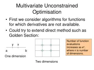
y x a Two dimensions Multivariate Unconstrained Optimisation • First we consider algorithms for functions for which derivatives are not available. • Could try to extend direct method such as Golden Section: Number of function evaluations increases as en, where n is number of dimensions. b One dimension
The Polytope Algorithm • This is a direct search method. • Also known as “simplex” method. • In n dimensional case, at each stage we have n+1 points x1, x2,…,xn+1 such that: F(x1) F(x2) F(xn+1) • The algorithm seeks to replace the worst point, xn+1, with a better one. • The xi lie at the vertices of an n-dimensional polytope.
The Polytope Algorithm 2 • The new point is formed by reflecting the worst point through the centroid of the best n vertices: • Mathematically the new point can be written: xr = c + (c-xn+1) where >0 is the reflection coefficient. • In two dimensions polytope is a triangle; in three dimensions it is a tetrahedron.
x1 (c-x3) c-x3 c xr x3 (worst point) x2 Polytope Example • For n = 2 we have three points at each step.
Detailed Polytope Algorithm • Evaluate F(xr)Fr. If F1 Fr Fn, then xr replaces xn+1. • If Fr< F1 then xr is new best point and we assume direction of reflection is “good” and attempt to expand polytope in that direction by defining the point, xe = c + (xr-c) where >1. If Fe< Fr then xe replaces xn+1; otherwise xr replaces xn+1.
Detailed Polytope Algorithm 2 • If Fr> Fn then the polytope is too big and we attempt to contract it by defining: xc = c + (xn+1-c) if Fr Fn+1 xc = c + (xr-c) if Fr < Fn+1 where 0<<1. If Fc< min(Fr,Fn+1) then xc replaces xn+1; otherwise a further contraction is done.
MATLAB Example Polytope >> banana = @(x)10*(x(2)-x(1)^2)^2+(1-x(1))^2; >> [x,fval] = fminsearch(banana,[-1.2, 1],optimset('Display','iter'))
Polytope Example • Start with equilateral triangle: x1 = (0,0) x2=(0,0.5) x3=(3,1)/4 • Take =1, =1.5, and =0.5
Polytope Example: Step 1 • Polytope is • Worst point is x1, c = (x2+ x3)/2 = (0.2165,0.375) • Relabel points: x3 x1, x1 x3 • xr = c + (c- x3) = (0.433,0.75) and F(xr)=3.6774 • F(xr)< F(x1) so xr is best point so try to expand. • xe = c + (xr-c) = (0.5413,0.9375) and F(xe)=3.1086 • F(xe)< F(xr) so accept expand
Polytope Example: Step 2 • Polytope is • Worst point is x2, c = (x1+ x3)/2 = (0.4871,0.5938) • Relabel points: x3 x1, x2 x3, x1 x2 • xr = c + (c- x3) = (0.9743,0.6875) and F(xr)=2.0093 • F(xr)< F(x1) so xr is best point so try to expand. • xe = c + (xr-c) = (1.2179,0.7344) and F(xe)=2.2837 • F(xe)>F(xr) so reject expand.
Polytope Example: Step 3 • Polytope is • Worst point is x2, c = (x1+ x3)/2 = (0.7578,0.8125) • Relabel points: x3 x1, x2 x3, x1 x2 • xr = c + (c- x3) = (1.0826,1.375) and F(xr)=3.1199 • F(xr)>F(x2) so polytope is too big. Need to contract. • xc = c + (xr-c) = (0.9202,1.0938) and F(xc)=2.2476 • F(xc)<F(xr) so accept contraction.
Polytope Example: Step 4 • Polytope is • Worst point is x2, c = (x1+ x3)/2 = (0.9472,0.8906) • Relabel points: x3 x2, x2 x3 • xr = c + (c-x3) = (1.3532,0.8438) and F(xr)=2.7671 • F(xr)>F(x2) so polytope is too big. Need to contract. • xc = c + (xr-c) = (1.1502,0.8672) and F(xc)=2.1391 • F(xc)<F(xr) so accept contraction.
Polytope Example: Step 5 • Polytope is • Worst point is x2, c = (x1+ x3)/2 = (1.0622,0.7773) • Relabel points: x3 x2, x2 x3 • xr = c + (c- x3) = (1.2043,0.4609) and F(xr)=2.6042 • F(xr)F(x3) so polytope is too big. Need to contract. • xc = c + (x3-c) = (0.9912,0.9355) and F(xc)=2.0143 • F(xc)<F(xr) so accept contraction.
Polytope Example: Step 6 • Polytope is • Worst point is x2, c = (x1+ x3)/2 = (0.9827,0.8117) • Relabel points: x3 x2, x2 x3 • xr = c + (c- x3) = (0.8153,0.7559) and F(xr)=2.1314 • F(xr)>F(x2) so polytope is too big. Need to contract. • xc = c + (xr-c) = (0.8990,0.7837) and F(xc)=2.0012 • F(xc)<F(xr) so accept contraction.
Polytope Example: Final Result • So after 6 steps the best estimate of the minimum is x = (0.8990,0.7837) for which F(x)=2.0012.
Alternating Variables Method • Start from point x = (a1, a2,…, an). • Take first variable x1, and minimise F(x1, a2,…, an) with respect to x1. This gives x1= a1. • Take second variable x2, and minimise F(a1, x2,…, an) with respect to x2. This gives x2= a2. • Continue with each variable in turn until minimum is reached.
AVM in Two Dimensions • Method of minimisation over each variable can be any univariate method. Start
AVM Example in 2D • Minimise F(x,y)=x2+y2+xy-2x-4y • Start at (0,0).
Definition of Gradient Vector • The gradient vector is: • The gradient vector is also written as F(x).
Definition of Hessian Matrix • The Hessian matrix is defined as: • The Hessian matrix is symmetric, and is also written as 2F(x).
Conditions for a Minimum of a Multivariate Function • |g(x*)| = 0. That is, all partial derivatives are zero. • G(x*) is positive definite. That is, xTG(x*)x > 0 for all vectors x0. • The second condition implies that the eigenvalues of G(x*) are strictly positive.
Stationary Points • If g(x*)=0 then x* is said to be a stationary point. • There are 3 types of stationary point: • Minimum, e.g., x2+y2 at (0,0) • Maximum, e.g., 1-x2-y2 at (0,0) • Saddle Point, e.g., x2-y2 at (0,0)
Definition: Level Surface • F(x)=constant defines a “level surface”. • For different values of the constant we generate different level surfaces. • For example, in 3-D suppose F(x,y,z) = x2/4 + y2/9 + z2/4 • F(x,y,z) = constant is an ellipsoid surface centred on the origin. • Thus, the level surfaces are a series of concentric ellipsoidal surfaces. • The gradient vector at point x is normal to the level surface passing through x.
Definition: Tangent Hyperplane • For a differentiable multivariate function, F, the tangent hyperplane at the point xt on the surface F(x)=constant is normal to the gradient vector.
Definition: Quadratic Function • If the Hessian matrix of F is constant then F is said to be a quadratic function. • In this case F can be expressed as: F(x) = (1/2)xTGx + cTx + for a constant matrix G, vector c, and scalar . • F(x) = Gx + c and 2F(x) = G.
Example Quadratic Function • F(x,y) = x2 + 2y2 + xy – x + 2y • Gradient vector is zero at stationary point, so Gx + c = 0 at stationary point • Need to solve Gx = -c to find stationary point: x* = G-1c x* = (6/7 -5/7)T
Hessian Matrix Again • We can predict the behaviour of a general nonlinear function near a stationary point, x*, by looking at the eigenvalues of the Hessian matrix. • Let uj and j denote the jth eigenvector and eigenvalue of G. • If j > 0 the function will increase as we move away from x* in direction uj. • If j < 0 the function will decrease as we move away from x* in direction uj. • If j = 0 the function will stay constant as we move away from x* in direction uj.
Example Again • 1 = 1.5858 and 2 = 4.4142, so F increases as we move away from the stationary point at (6/7 -5/7)T. • So the stationary point is a minimum.
Example in 4D • In MATLAB: >> c = [-1 2 3 4]’; >>G = [2 1 0 2; 1 2 -1 3; 0 -1 4 1; 2 3 1 -2]; >>x = G\(-c) >>[u,lambda] = eigs(G)
Descent Methods • Seek a general algorithm for unconstrained minimisation of a smooth multivariate function. • Require that F decreases at each iteration. • A method that imposes this type of condition is called a descent method.
A General Descent Algorithm Let xk be current iterate. • If converged then quit; xk is estimate of minimum. • Compute a nonzero vector pk giving direction of search. • Compute a positive scalar step length, k for which F(xk+ k pk) < F(xk). • New estimate of minimum is xk+1 = xk+ kpk. Increment k by 1, and go to step 1.
Method of Steepest Descent • Direction in which F decreases most steeply is -F, so we use this as the search direction. • New iterate is xk+1 = xk - kF, where k is non-negative scalar chosen so that xk+1 is the minimum point along the line from xk in the direction -F. • Thus, k minimises F(xk - F) with respect to .
Steepest Descent Algorithm • Initialise: x0, k=0 • Loop: u = F(xk) if |u|=0 then quit else minimise h()=F(xk- u) to get k xk+1 = xk- ku k = k+1 if (not finished) go to Loop
Example • F(x,y) = x3 + y3 - 2x2 + 3y2 - 8 • F(x,y) = 0 gives 3x2-4x=0 so x = 0 or 4/3; and, 3y2+6y=0 so y=0 or -2.
Solve with Steepest Descent • Take x0 = (1 -1)T, then F(x0)=(-1 -3)T. • h()F(x0- F(x0)) = F(1+,-1+3) = (1+)3+(3-1)3-2(1+)2+3(3-1)2-8 • Minimise h() with respect to . h/ = 3(1+)2+9(3-1)2-4(1+)+18(3-1) = 842 + 2 -10 = 0 • So = 1/3 or -5/14. must be nonnegative so = 1/3.
Solve with Steepest Descent • x1 = x0 - F(x0) = (1 -1)T – (-1/3 -1)T = (4/3 0)T. • This is the exact minimum. • We were lucky that the search direction at x0 points directly towards (4/3 0)T. • Usually we would need to do more than one iteration to get a good solution.
Newton’s Method • Approximate F locally by a quadratic function and minimise this exactly. • Taylor’s Theorem: F(x) F(xk)+(g(xk))T(x-xk)+ (1/2)(x-xk)TG(xk)(x-xk) = F(xk)-(g(xk))Txk+ (1/2)xkTG(xk)xk+ (g(xk)-G(xk)xk)Tx+(1/2)xTG(xk)x • RHS is minimum when g(xk) – G(xk)xk+G(xk)xk+1=0 • So xk+1= xk – [G(xk)]-1g(xk) Search direction is -[G(xk)]-1g(xk) and step length is 1.
Newton’s Method Example • Rosenbrock’s function: F(x,y) = 10(y-x2)2 + (1-x)2 • Use Newton’s Method starting at (-1.2 1)T.
MATLAB Solution >> F=@(x,y)10*(y-x^2)^2+(1-x)^2 >>fgrad1=@(x,y)-40*x*(y-x^2)-2*(1-x) >>fgrad2=@(x,y)20*(y-x^2) >>G11=@(x,y)120*x^2-40*y+2 >>x=[-1.2;1] >>x=x-inv([G11(x(1),x(2)) -40*x(1);-40*x(1) 20])*[fgrad1(x(1),x(2)) fgrad2(x(1),x(2))]’
Notes on Newton’s Method • Newton’s Method converges quadratically if the quadratic model is a good fit to the objective function. • Problems arise if the quadratic model is not a good fit outside a small neighbourhood of the current point.