Advances in Macroscopic Quantum Coherence: Experiments and Theoretical Insights
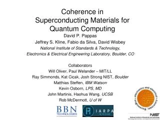
This report summarizes the advancements in the field of Macroscopic Quantum Coherence (MQC) spearheaded by A. Leggett's proposal. It discusses the implementation of quantum coherence in superconducting circuits, specifically utilizing rf-SQUIDs at Università di Roma “La Sapienza.” Key topics include experimental measurements of quantum effects, non-invasive measurement techniques, quantum dissipation, and Rabi oscillations. The report also highlights ongoing developments in quantum computation on both a local and global scale, solidifying the relevance of MQC in contemporary physics.

Advances in Macroscopic Quantum Coherence: Experiments and Theoretical Insights
E N D
Presentation Transcript
MQC Macroscopic Quantum Coherence Carlo Cosmelli, G. Diambrini Palazzi Dipartimento di Fisica, Universita`di Roma “La Sapienza” Istituto Nazionale di Fisica Nucleare Commissione Nazionale II- Relazione Finale – 19.11.2003
Sommario • Introduzione storica, la proposta di A. Leggett • MQC con rf SQUID, MQC a Roma • Misure e risultati intermedi: • Il dispositivo • (Il Laser switch) • Misure non invasive • Misure di dissipazione quantistica • Misura delle oscillazioni di Rabi: MQC con un dc SQUID • Sviluppi a Roma e nel mondo: la computazione quantistica
Quantum Mechanics (QM) Classical Mechanics (CM) Superposition Principle Macrorealism 1935 - Einstein, Podolski, Rosen : The description of (microscopic) reality given by the quantum wave function is not complete 1964 - J. Bell : We can imagine a two particle experiment giving different results for CM (locality) or QM (non locality). 1972 - A. Aspect : Bell experiment with two polarized photons. Violation of Bell inequalities. Non locality. 1985 - A. Leggett : Can we have a non classical behavior in a macroscopic system? MQC = Macroscopic Quantum Coherence
The double well potential: Leggett 1985: propose a device having a double well potential (a SQUID) to create a double well potential
U(f) L> R> f I rf SQUID states: L & R ES EA
P(t) 1 1/2 0 t MQC (Rabi Oscillations) :QM vs. MR : P(L,tL, t=0) cos2 t where = tunnelling frequency between wells
Il gruppo MQC: (in giallo i membri temporanei) • Università La Sapienza • G. Diambrini Palazzi, C. Cosmelli, F. Chiarello, D. Fargion, INFN Roma • Istituto Fotonica e Nanotecnologie – CNR, Roma • M.G. Castellano, R. Leoni, G. Torrioli, INFN Roma • Università dell’Aquila • P. Carelli, G. Rotoli,INFN G. C. Sasso/Tor Vergata • Università di Tor Vergata • M. Cirillo, INFN Tor Vergata • Istituto di Cibernetica – CNR- Napoli • R. Cristiano, G. Frunzio, B.Ruggiero, P. Silvestrini, INFN Napoli • Istituto Regina Elena –Centro Ricerche • L. Chiatti • 9 Laureandi, 2 Dottorandi
Organizzazione: • Roma – CNR, L’Aquila • Progettazione dispositivi superconduttori • Realizzazione dispositivi • Test preliminari a T= 4.2 K • Roma – La Sapienza • Simulazioni • Test a rf a T=4.2 K • Test a T<100mK • Analisi Risultati
I L (superconducting) + Josephson Junction = SQUID MQC can be realized with a SQUID • N : 1010 Cooper pairs; I 1-10 A • The system dynamics can be controlled and measured in the classical regime ( J. Clarke, 1987). • The intrinsic dissipation can be made negligible [ exp(-Tc/T)] • The system Hamiltonian is non linear. • The effect can be seen in reasonable short times (nss).
Il potenziale dello SQUID (rf-dc-jj...) • La pendenza media può essere variata dall’esterno (corrente-flusso) • Varia l’altezza della barriera di potenziale • Variano le frequenze di tunneling • Variano le distanze fra i vari livelli energetici E1> E2> E3 analogamente variano le risonanze con i livelli energetici delle buche adiacenti
P(t) 1 1/2 0 t Experimental Requirements • Suppose we want to observe oscillations from one well to the other with tunneling frequency • The tunneling probability is exponentially depressed by dissipation (Caldeira, Leggett, Garg) • P(t) =1/2[1+cos (t) exp (- t)] low temperature :T< 20mK low dissipation : R > 1 M
Rome group Leiden cryogenics Low Temperature: 3He-4He dilution refrigerator • T=9 mK, power= 200 W at 120 mK • 3 -metal shields (> 40 dB between dc and 100 Hz) • 2 Al shields (> 90 dB at 1 MHz) • Set of Helmoltz coils 1.5x1.5x1.5 m3 (34 dB attenuation of Earth magnetic field within 1 dm3) • Magnetically levitated turbo pump • Vibration Isolation platform, frequency cut ~1 Hz. • Sample immersed in the liquid 3He-4He mixture.
Scheme of the experimental SQUID system dc bias laser SQUID Switch Vout(f) SQUID rf rf bias SQUID Amplifier
dc-SQUID amplifier coils tunable rf-SQUID readout hysteretic dc-SQUID Chip for the MQC experiment 100m
Lo SQUID di letturaper effettuare misure non invasive (un dc SQUID)
vout vout Ib Ib FR FL Utilizzo di un dc-SQUID per la misura non invasiva dello SQUID rf Il dc SQUID viene “acceso” da un impulso di corrente, che lo mantiene nello stato superconduttore, V=0 = R Vout= 0 = L Vout 0 NIM: Non Invasive Measurement Misura Invasiva: si scarta
Sensibilità: larghezza della transizione V=0 V0 Switch probability of hysteretic dc-SQUID as a function of applied magnetic flux and temperature
Detection efficiency:prediction: 98%measured: 98% current bias of hysteretic SQUID P voltage output of hysteretic SQUID voltage output of SQUID magnetometer F (mF0) optimal bias point
The Problem of Dissipation • Shield all cables from high temperature signals • Shield from external e.m. fields • Shield from mechanical vibrations • Leave only intrinsic dissipation • Measure overall dissipation.
Misure di Energy Level Quantization per valutare la dissipazione intrinseca del sistema Diminuendo l’altezza della barriera si provoca l’escape per tunneling dei vari livelli energetici: si misura =1/ in funzione dello sbilanciamento Dalla forma di si calcola il valore della dissipazione effettiva del sistema 2c
(s-1) 105 103 101 10-1 .964 .968 .972 .976 I/Ic Experimental results Escape rate for a Josephson junction T= 20 mK - R 1 M (C. Cosmelli et al. Phys. Rev. 1998) (s-1) Escape rate for an rf SQUID T=35mK - R 4 M 103 101 10-1 -.48 -.47 -.46 (C. Cosmelli et al. Phys. Rev. Lett. 1999) e0
Energy level quantization in thermal regime fast sweeping of the current, non-stationary regime, T > Tcrossover T=1.3 K (IC-Napoli)
Misura delle oscillazioni di Rabiin un sistema macroscopico(un dc SQUID non un rf SQUID!)
Continuous microwaves at fixed frequency f • Different fluxes Fx • For each flux: sequence of current pulses • For each pulse: voltage read-out (0 or 2.7mV) • Switching probability P at different Fx: • switching curve • peaks Test with continuous microwaves - I
Microwaves can excite the system when f=(En-E0)h • To find the peaks positions: • Hamiltonian Eigenenergies E0, E1, E2, ... • Fluxes to have f= (En-E0)h Peaks at the expected positions Experimental values f = 14.999 GHz Ipulse = 5.5 mA Dtpulse = 50 ns I0max = 19 mA Ctot = 1.1 pF L = 12 pH T = 60 mK Test with continuos microwaves - II
wave pulse Test with short pulses of microwaves • Flux fixed on the second peak at Fx = 0.405 F0 • A short (100 ns – 500 ns) pulse of microwaves is applied to the dc SQUID • A reading current pulse of proper shape is send to the dc SQUID • The voltage across the SQUID (0 or 2,7 mV) is read at a proper time.
The plot represents the probability P[ |1>,t ; |0>, 0] as a function of the microwave pulse duration Dt Systemparameters f = 14.999 GHz hf/KB=720 mK Fx = 0.405 F0 Ipulse = 5.5 mA Dtpulse = 50 ns I0max = 19 mA Ctot = 1.1 pF L = 12 pH T = 60 mK Results: Rabi Oscillations on a Macroscopic System • frequency of oscillations =7,4 MHz • Decoherence time = 150 ns • Tc (thermal/quantum regime) 100 mK
World state of art – observation of coherence on macroscopic systems (SQUIDs) Work in progress: Berkeley (USA), IBM (USA)
peak and dip under -wave resonance between photon and energy spacing between lowest quantum states level repulsion
Sviluppi futuri: SQC Superconducting Quantum Computing SQC è attualmente finanziato in gruppo V – end 2004
Quantum computing vs. Classical Computing Quantum computing vs. Classical Computing bit qubit bit qubit { } { } { } { } Classical computer Quantum computer Classical computer Quantum computer º º º º 0 |0> 1 bit two states 1 qubit |0> + |1> a b 1 ¥ ¥ states states |1> It is probabilistic reading It is deterministic reading qubit gives the value a bit gives always the value of its state |0> with probability a 0 or 1 |1> with probability b The output is 0 or 1 : a : : 2 2 The output is 0 or 1 Carlo Cosmelli, Roma
Quantum Computer Classical computer Factorization times: QC power • 1977 M. Gardner propose the factorization of a 129 bit number • 1994 The number is factorized: 1000 Workstations – 8 months
Potential i0 : single junction critical current Tunable system A hysteretic dc SQUID as a qubit system “Artificial atom” - Qubit states: |E0>, |E1> - Manipulation: Rabi oscillations - Read-out: current pulse to reduce DU in order to have escape from E1 and not from E0
Potential Tunable system A double rf SQUID as a qubit system “Pseudo-spin ½ system” - Qubit states: |FL>, |FR> - Manipulation: Rabi oscillations, external fluxes variations - Read-out: SQUID magnetometer or flux comparator
Quantum Information Technology:Public Founding, next 5 years • Japan 20 M€/year • Europe (EC) 7 M€/year + Single States • USA 6 M€/year + Universities Includes all QIT (Solid State, Photons, Quantum Dots, Atoms, Semiconductors, Molecules, ....) for experimental and theoretical research.