Disturbance Rejection
This text delves into the concept of disturbance rejection in control systems, emphasizing its importance in maintaining system stability. It explores key questions such as the conditions under which output approaches zero, the implications for hardware, and how disturbance rejection is achieved through specific input and hardware configurations. The Final Value Theorem is also examined, highlighting requirements for poles in the right half plane and complex poles. The document serves as both a foundational reference and a homework assignment related to disturbance rejection principles.

Disturbance Rejection
E N D
Presentation Transcript
Disturbance Rejection Disturbances only mentioned on page 3 of Ogata Disturbance Rejection
Disturbance Rejection R(s)=0 N(s)=0 Disturbance Rejection
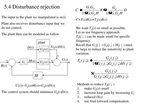
Red is input signal Blue is specified hardware Green is unspecified hardware When will A be close to zero? When will A be exactly zero? What does this mean for the hardware? Why? Disturbance Rejection Homework 1 and 2 are now assigned. Disturbance Rejection
Final Value Theorem • We have been performing a particular computation over-and-over again. Assume that Y(s) has • no poles in the RHP, and • has no complex poles on the imaginary axis, except for • perhaps a simple pole at the origin, then This is called the Final Value Theorem. See page 233 of FC&N See pp. 76 of DS&W See page19 of FE Reference, 2nd to last entry of table Disturbance Rejection
Proof of FVT Assumptions as on previous slide. End of Proof. Notice the similarity in the work we have done several time. Many (most?) Theorems come from such observations. Notice that if Y(s) does not have a pole at s=0, then A evaluates to 0. Disturbance Rejection