Download
1 / 22
220 likes | 316 Vues
This paper explores the performance limitations and optimization methods for disturbance rejection using indirect control in the context of chemical engineering. It discusses interpolation and derivative constraints, comparing direct and indirect control approaches. The study unifies treatment of different closed-loop functions and provides specific assumptions and results regarding unstable poles and zeros. Practical implications and examples are examined, highlighting the importance of closely correlated signals and the potential of feedforward controllers to overcome limitations. The research emphasizes achieving optimal performance while managing sensitivity to disturbances and uncertainties.

E N D
Limits of Disturbance Rejection using Indirect Control Vinay Kariwala* and Sigurd Skogestad Department of Chemical Engineering NTNU, Trondheim, Norway skoge@chemeng.ntnu.no * From Jan. 2006: Nanyang Technological University (NTU), Singapore
Outline • Motivation • Objectives • Interpolation constraints • Performance limits • Comparison with direct control • Feedback + Feedforward control
d Gd z u K G - y = z “Direct” Control Unstable (RHP) zeros αi in G limit disturbance rejection: interpolation constraint
Compositions cannot be measured or are available infrequently Problem In many practical problems, • Primary controlled variable z not available Need to consider “Indirect control”
d Gd z G Gdy u K Gy - y Indirect Control Indirect control: Control y to achieve good performance for z Primary objective paper: Derive limits on disturbance rejection for indirect control
Related work • Bounds on various closed loop functions available • S, T – Chen (2000), etc. • KSGd – Kariwala et al. (2005), etc. • Special cases of indirect control Secondary objective: Unify treatment of different closed loop functions
Main Assumptions (mostly technical) • Unstable poles of G and Gdy– also appear in Gy • All signals scalar • Unstable poles and zeros are non-repeated • G and Gdy - no common unstable poles and zeros
a • Interpolation constraints • Derivative constraints Nevanlinna-Pick Interpolation Theory Parameterizes all rational functions with Useful for characterizing achievable performance
If are unstable zeros of G If are unstable zeros of Gdy Indirect control: Interpolation Constraints Need to avoid unstable (RHP) pole-zero cancellations same as for direct control
If are unstable poles of Gy that are shared with G If are unstable poles of Gy that are shared with Gdy If are unstable poles of Gy not shared with G and Gdy - stable version (poles mirrored in LHP) More new interpolation Constraints
Reason: Derivative is also fixed Derivative Interpolation Constraint Special case: Control effort required for stabilization Bound due to interpolation constraint Very conservative: Should be:
optimal achievable performance optimal achievable performance Main results: Limit of Performance, indirect control Let v include all unstable poles and zeros: Derivative constraint neglected, Exact bound in paper
G and Gdy have no unstable poles • or has transmission zeros at these points and “Perfect” Indirect Control possible when: • G and Gdy have no unstable zeros • or Gd evaluated at these points is zero and • Gyhas no extra unstable poles
Zeros of G Direct Control vs Indirect Control • Poles of G + (Possible) derivative constraint Practical consequence: To avoid large Tzd, y and z need to be “closely correlated” if the plant is unstable
Indirect control The required change in u for stabilization may make z sensitive to disturbances Exception: Tzd(gammak) close to 0 because y and z are “closely correlated” Example case with no problem : “cascade control” In this case: z = G2 y, so a and y are closely correlated. Get Gd = G2 Gdy and G = G2 Gy, and we find that the above bound is zero
Direct Indirect Case Stable system 0.5 0.5 Unstable system 1.5 15.35 Extra unstable pole of Gy - 51.95 Simple Example
d M Gd z G K2 Gdy u K1 Gy - y Feedback + Feedforward Control Disturbance measured (M)
Feedback + Feedforward Control • No limitation due to • Unstable zeros of Gdy unless M has zeros at same points • Unstable poles of G and Gdy • Limitation due to • Unstable zeros of G • Extra unstable poles of Gy, but no derivative constraint • + Possible limitation due to uncertainty
FB+FF FB+FF 0.5 0.5 0.5 0.5 - 0.68 Simple Example (continued) Indirect Case Direct FB FB Stable system 0.5 0.5 Unstable system 1.5 15.35 Extra unstable pole of Gy - 51.95
Conclusions • Performance limitations • Interpolation constraint, derivative constraint • and optimal achievable performance • Indirect control vs. direct control • No additional fundamental limitation for stable plants • Unstable plants may impose disturbance sensitivity • Feedforward controller can overcome limitations • but will add sensitivity to uncertainty
Limits of Disturbance Rejection using Indirect Control Vinay Kariwala* and Sigurd Skogestad Department of Chemical Engineering NTNU, Trondheim, Norway skoge@chemeng.ntnu.no * From Jan. 2006: Nanyang Technological University (NTU), Singapore