Download
1 / 9
110 likes | 250 Vues
plant. G d ( s ) D ( s ). D ( s ). G d (s). +. C ( s ). +. M ( s ). +. G c. G p ( s ). R ( s ). –. H. 5.4 Disturbance rejection. The input to the plant we manipulated is m ( t ). Plant also receives disturbance input that we do not control. The plant then can be modeled as follow.

E N D
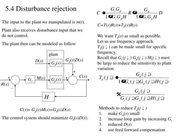
plant Gd(s)D(s) D(s) Gd(s) + C(s) + M(s) + Gc Gp(s) R(s) – H 5.4 Disturbance rejection The input to the plant we manipulated is m(t). Plant also receives disturbance input that we do not control. The plant then can be modeled as follow C=T(s)R(s)+Td(s)R(s) We want Td(s) as small as possible. Let us use frequency approach. Td(j) can be made small for specific frequency. Recall that Gc(j) Gp(j) H(j) must be large to reduce the sensitivity to plant variation. • Methods to reduce Td(j) • make Gd(s) small • increase loop gain by increasing Gc • reduced D(s) • use feed forward compensation C(s)= Gp(s)M(s)+Gd(s)D(s) The control system should minimize Gd(s)D(s).
D(s) plant Gd(s)D(s) Gd(s) Gcd(s) + – C(s) + M(s) + Gc Gp(s) R(s) – H 5.4 Disturbance rejection Feedforward compensation Feedforward compensation can be applied if the disturbance can be measured. We choose Gcd(s)Gc(s) such that Td(s) will as small as possible. The addition of compensator Gcd(s) does not effect T(s) the TF from R(s) to C(s) but does for Td(s)
E(s) M(s) C(s) + Gc Gp(s) R(s) – The steady state error ess is defined as 5.5 Steady State Accuracy Step input, R(s) = 1/s hence We will examine the steady state error ess for different system types. Assume H=1. hence For N = 0 then Kp = Kp and ess=1/(1+ Kp) For N > 0 then Kp = and ess= 0. Ramp input, R(s) = 1/s2 hence We can express For N = 0 then Kv = 0 and ess= For N = 1 then Kv = Kv and ess= 1/ Kv For N > 1 then Kv = and ess= 0 N is integer and the system is called system type N. N is also the number of integrator in GcGp we will demonstrate its importance
The steady state error ess system typeinput N 1/s 1/s2 1/s3 0 1/(1+KP) 1 0 1/Kv ess 2 0 0 1/Ka Kp is called position error constant Kv is called velocity error constant Kv is called acceleration error constant Plot of ramp responses of different type system 5.5 Steady State Accuracy Parabolic input, R(s) = 1/s3 hence ess For N < 2 then Kv = 0 and ess= For N = 2 then Ka = Ka and ess= 1/ Ka For N > 2 then Kv = and ess= 0 type 0 system ess type 1 system type 2 system
+ R(s) – H Ru(s) E(s) C(s) + – 5.5 Steady State Accuracy Non-unity-Gain feedback The non-unity gain feedback above has equivalent block diagram as follow provided that H(s) is constant. Where Ru(s) = R(s)/H. Hence the position, velocity, and acceleration error constant can be calculated in the same manner
Disturbance Input Error Let us consider steady state error due to disturbance input. Recall that the output of disturbed plant C(s) =T(s)R(s)+Td(s)C(s)=Cr(s)+Cd(s) The system error is then e(t)= r(t) –c(t) =[r(t) –cr(t)] –cd(t) = er(t) + ed(t) where er(t) is the error we’ve just considered We see that ed(t)= –cd(t) and we want it to be small. The steady state of ed(t) is (3) (1) (2) To draw general conclusion we must consider the type number of Gp(s) Gc(s) and Gd(s). where (assuming H = 1) Let us model the disturbance input as step function, D(s)=B/s. From (1) we have
The factor is called the modes TRANSIENT RESPONSE The system TF can be written as Here cr(t) is the forced response and the rest is the natural response or the transient response For stable system the natural response will decay to zero. The way it decays to zero is important. The transient response ctr(t) is The response for input R(s) is The nature or form of each term is determined by the pole location of pi. Where Cr(s) is the part that originate from the poles of R(s) The inverse LT of this equation is
For each real pole, a time constant is associated with it with the value TRANSIENT RESPONSE The amplitude of each term is For each set complex conjugate poles of values Thus the amplitude of each term determined by other pole location, the numerator polynomial, and the input function. For higher order system it is difficult to make general assertion, however we can consider the nature of each term of this response. there is associated damping ratio , a natural frequency n , and time constant i =1/n. If there is one real dominant pole the system responds essentially as 1st order system. If there is dominant complex poles then the system respond essentially as 2nd order system.
|T()| (1). B CLOSED LOOP FREQUENCY RESPONSE The input output characteristics are determined by CL frequency response T(0) is the system dc gain. This values determines the steady state error. If we evaluate (1) for small we see how the system will follow for slow varying input. The bandwidth can be evaluated form (1). Large bandwidth indicate fast system response. The presence of any peaks, which denotes resonance, give indication of the overshoot or decaying oscillation