Eclipse Simulation Data Visualization Tool
iGridView is a 2D box view for Eclipse simulation data, allowing tracking, modification, calculation, and export of properties. Load input, initialization, and recurrent data, view properties across layers, group layers, set display options, and more.

Eclipse Simulation Data Visualization Tool
E N D
Presentation Transcript
iGridView description Version 2.0
Introduction • IGridView is a 2D box view of Eclipse simulation data. • Three types of grid data can be loaded and viewed: • Input properties • Initialized by Eclipse properties • Recurrent Eclipse simulation properties • The properties is shown in 2D box top view with color and value in each cell. Properties in different simulation layer can be viewed by selecting a layer or navigating thru them. • Multiple layer can be grouped by holding Shift/Ctrl key while selecting layer. The properties for selected layers will be summed up or averaged according to selected Option. • Well completion (if any) is also displayed. • IGridView allows to keep track (and set) modification to the model. • New properties can be calculated and exported.
Requirement • For loading input data file: • All keywords have to be on a line by themselves.: Example: EQUIL 3 TABLES 20 NODES IN EACH FIELD 14:32 2 JAN 90 7100.00 3814.70 7500.00 0.00000 7100.00 0.00000 1 0 5 / EQUIL --3 TABLES 20 NODES IN EACH FIELD 14:32 2 JAN 90 7100.00 3814.70 7500.00 0.00000 7100.00 0.00000 1 0 5 / • No space is allowed in string variable/no blank string variable. Example: WELSPECS 'L 1 ', ‘ ', 14, 8, 7300.00, 'OIL‘ / WELSPECS 'L_1 ', ‘GROUP1', 14, 8, 7300.00, 'OIL‘ / Not OK OK Not OK: space in well name, blank group name OK
Requirement • For loading Init data. • .INIT file must be presented (requested by keyword INIT in grid section of the eclipse run. • For loading Recurrent data. • .RSSPEC and .UNRST file (. X0001, .X0002, … files in case of un-unified data) must be presented.
iGridView Menu 5- Properties manager: Select for view, copy, paste, export 8- Set the modification to properties 9- Modify the modifers 1-Load a Simulation Case 3-Set display option 2-Add New Case 4-Set the filter 6-Set the Cell Probe 7- Layer and Time navigator 10- Export modifier to Eclipse format 11- Properties calculator
1 & 2 - Load/Add Simulation Case • Click on Load Data, Window Explorer will appear to let the user select the simulation case to load. Program will check for .INIT and restart files and let user select the type of data to load as shown on the right. • One case has to be Loaded before other cases can be added. • Unlimited cases can be loaded (depend on available free computer memory)
3 – Set Display Option Option to show the properties when multiple layer is selected. Option to Color the cell Create the net mobile oil thickness for recurrent simulation data. User can select the case, specify the layer grouping scheme, the option for calculation and click “Create Mobile Oil” for automatically generating the mobile oil thickness. On the above setting, mobile oil thickness will be created for case 50x50x50M, grouped for layer 1 to 2, 3 to 4, and 5 to 6. The MOB_OIL properties will be shown on list of recurrent properties. Threshold of transmissibility barrier: multiplier less than Threshold 2 will be shown as solid line, between the Threshold 1 and Threshold 2 will be shown as dotted thin line.
5 - Display Properties Select loaded case Select type of data Select layer Multiple layers can be selected by holding Shift/Ctrl while selecting. Select props Viewing option (for Input props only): A- View original array B- View after applying all modification keywords C- View ratio of B to A Select timestep if available Copy a props for pasting into other cases Export selected property (ASCII Eclipse format) Import Properties (ASCII Eclipse format) into this case.
Example of viewing option 1 • Option 1: View Original Data (PORO, layer 1). Note the well completion shown in the grid as the diagonal cross.
Example of viewing option 2 • Option 2: View with all changes (PORO, layer 1). Some shown values are different from previous view.
Example of viewing option 3 • Option 3: View Ratio of change (PORO, layer 1). A rectangle at the center shown value of 1.05, which is modification made to PORO.
4 - Filter Turn on/off the use of filter Select type of data Turn on/off the use of inverted filter Select props Select timestep if availble Turn on/off the use of new color scheme for new filter Update min For discrete props: use list of value to filter data Update max List of all value (discrete props: PVTNUM, SATNUM,…) Clear all filters Apply selected filter
6- Cell Probing Selecting type of data for probing Select height above OWC and PERMX for probing. (When loading Input data, height above OWC and GOC will be generated) Highlight the props to be selected Select highlighted props for probing deSelect highlighted props from probing list Select simulated timestep (if available) Delete all props in probe list Turn on/off the cell probing Option for multicells selection
Example of Cell Probing • When the Probe is turned on, clicking on any cell will display a small window showing probed valued. • Click outside of view panel to hide the Probing window. • Turn the Cell Probe off if no probing is desired.
8 - Set Modifier • When click on “Set Modifier” Input box will display, asking to select the region user want to modify (using mouse selection). • Multiple regions is selected by holding the Ctrl at the same time as mouse selection. • On this example, three regions are selected for introducing the barrier (shown with dotted line and also by text in the input box).
8 - Set Modifier Select props to modify • Upon selecting the modified region, new window appears for selecting appropriate option. • In this example on the right, a sealed barrier (Multiplier to TRANXY of 0) is introduced follow the + direction of selected regions. • Click OK and the change will be shown on display panel as a solid line. Enter value of modifier Option for directional props (perm, trans) Scope of change (in K direction) Option for applying the transsmissibility barrier: follow J- or J+ Modification keyword Option for fluid region
Example of Setting the Transsmissibility barrier • A solid thick line is shown (as Transmissibility multiplier to 0 is entered.) If the multiplier is greater than transsmissibility threshold 1 (entered in Option), then no barrier is shown. If it is between threshold 1 and threshold 2, dotted thin line will be shown.
9 – Edit Modifiers • Modifers entered in Eclipse dataset or interactively entered using Set Modifers can be view and edit upon clicking “Edit Modifers” • A window appears showing list of all modifications. • If the list is extensive, view by predefined category can be selected (PORO, PERMXYZ, TRANXYZ) • Selecting any modifier and it will shown the corresponding region in View panel. • User can delete, or change the values of modification.
Edit Modifier Example • This example show the View Panel when user select one modification and select “Edit”. • New window appears allowing user to change the value and scope of modifier.
10 - Export Modifier • Interactively set modifier can be exported as a include file for use in Eclipse by clicking Export Modifier and select the modifiers to be exported. • Upon entering description, include file(s) will be generated (if TRANSXYZ is selected, it will be exported to a separated file with suffix _ED (to be included in EDIT section), otherwise they will be exported to file with suffix _GR (to be included in GRID section).
11 - Calculator • Simple properties calculator can be invoked to calculate new properties. In this example, property TEST=PORO*2 is calculated. • Calculated props will be attached to Input data type. They can be deleted or rename. They can be selected for viewing or use as filter in the same manner as other properties. History of calculation in current working session Type of new properties Name of new properties Excel-type expression. Existing properties can be included by selecting in properties selector window and click ^ button. Insert selected props into Expression List of new properties. These props can be renamed or deleted.