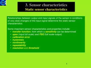
3. Sensor characteristics Static sensor characteristics
3. Sensor characteristics Static sensor characteristics. Relationships between output and input signals of the sensor in conditions of very slow changes of the input signal determine the static sensor characteristics. Some important sensor characteristics and properties include:

3. Sensor characteristics Static sensor characteristics
E N D
Presentation Transcript
3. Sensor characteristics Static sensor characteristics Relationships between output and input signals of the sensor in conditions of very slow changes of the input signal determine the static sensor characteristics. Some important sensor characteristics and properties include: • transfer function, from which a sensitivity can be determined • span (input full scale) and FSO (full scale output) • calibration error • hysteresis • nonlinearity • repeatability • resolution and threshold
Transfer function An ideal relationship between stimulus (input) x and sensor output y is called transfer function. The simplest is a linear relationship given by equation y = a + bx (3.1) The slope b is called sensitivity and a (intercept) – the output at zero input. Output signal is mostly of electrical nature, as voltage, current, resistance. Other transfer functions are often approximated by: logarithmic function y = a + b lnx (3.2) exponential function y = a ekx (3.3) power function y = ao + a1xc (3.4) In many cases none of above approximatios fit sufficiently well and higher order polynomials can be employed. For nonlinear transfer function the sensitivity is defined as S = dy/dx (3.5) and depends on the input value x.
Sensitivity Measurement error Δx of quantity X for a given Δy can be small enough for a high sensitivity. Over a limited range, within specified accuracy limits, the nonlinear transfer function can be modeled by straight lines (piece-wise approximation). For these linear approximations the sensitivity can be calculated by S = Δy/Δx
Span and full scale output (FSO) An input full scale or span is determined by a dynamic range of stimuli which may be converted by a sensor,without unacceptably high inaccuracy. For a very broad range of input stimuli, it can be expressed in decibels, defined by using the logarithmic scale. By using decibel scale the signal amplitudes are represented by much smaller numbers. For power a decibel is defined as ten times the log of the ratio of powers 1dB = 10 log(P/P0) Similarly for the case of voltage (current, pressure) one introduces 1dB = 20 log(V2/V1) Full scale output (FSO) is the difference between ouput signals for maximum and minimum stimuli respectively. This must include deviations from the ideal transfer function, specified by ±Δ.
Calibration error Calibration error is determined by innacuracy permitted by a manufacturer after calibration of a sensor in the factory. To determine the slope and intercept of the function one applies two stimuli x1 and x2 and the sensor responds with A1 and A2. The higher signal is measured with error – Δ. This results in the error in intercept (new intercept a1, real a) δa = a1 – a = Δ /(x2-x1) and in the error of the slope • δb = Δ /(x2-x1)
D y - Max. difference at output for specified input D x Hysteresis This is a deviation of the sensor output, when it is approached from different directions.
y ± % FSO Best straight line x Nonlinearity This error is specified for sensors, when the nonlinear transfer function is approximated by a straight line. It is a maximum deviation of a real transfer function from the straight line and can be specified in % of FSO. The approximated line can be drawn as the so called „best straight line” which is a line midway between two parallel lines envelpoing output values of a real transfer function. Another method is based on the least squares procedure.
y Cycle 1 Cycle 2 D Δ - max. difference between output readings for the same direction x Repeatability This error is caused by sensor instability and can be expressed as the maximum difference between output readings as determined by two calibration cycles, given in % of FSO. δr = Δ / FSO
y D resolution threshold x Rsolution and threshold Threshold is the smallest increment of stimulus which gives noticeable change in output. Resolution is the step change at output during continuous change of input.
Dynamic characteristics When the transducing system consists of linear elements dissipating and accumulating energy, then the dependence between stimulus x and output signal y can be written as equality of two differential equations A0y + A1y(1) + A2y(2) + ... + Any(n) = k (B0x + B1x(1) + B2x(2) + ... Bmx(m)) (1) y(1) – 1-st derivative vs. time k – static sensitivity of a transducer m ≤ n Eq. (1) can be transformed by the Laplace integral transformation (2) where s = σ + jω
Integrating (2) by parts it is easy to show that (3) Transforming eq. (1) using Laplace transformation, with the help of property (3) and with zero initial conditions one obtains the expression for operator transmittance of the sensor In effect we transfer from differential to algebraic equations. The analysis of an operator transmittance is particularly useful when the transducer is built as a measurement chain. The response y(t) one obtains applying reverse Laplace transformation.
x(t) 1 x(t) = (t) 0 for t < 0 1 1 (t) = ³ 0 1 for t t Excitation by a step-function The response of a sensor system depends on its type. It can be an inercial system, which consists of accumulation elements of one type (accumulating kinetic or potencial energy) and dissipating elements.
An example of inertial transducer Resistance thermometer immersed in the liquid of elevated temperature Electric analog L{1(t)} = X(s) = 1/s Inertial element of the 1-st order
Inertial element of the 1-st order, calculation of operator transmittance Therefore
Time response to the step function of inertial element of the 1-st order τ – time constant, a measure of sensor thermal inertia; For electric analogue τ = RC what means for t = τ 63% of a steady value. For t = 3τ one gets 95% of a steady value.
Response to the step function of an inertial element of higher order t95 - 95% response time Δt = t90 – t10 – rise time τ = t63 – time constant Insertion of a thermometer into an insulating sheath transforms it into an inertial element of higher order.
Response of an oscillating system to the step function 1 –oscillations 2 – critical damping 3 – overdamping Tranducer of the oscillation type consists of accumulating elements of both types and dissipating elements. Mechanical analogue is a damped spring oscillator (the spring accumulates potential energy, the mass – kinetic energy, energy is dissipated by friction). Electric analogue is an RLC circuit.
Mechanic analogue Electric analogue
Transmitance of the oscillating system The denominator of expression for transmittancecan have: • Two real roots overdamping 2) One real root critical damping 3) Two complex roots underdamping (oscillations) After inverse Laplace transformation one gets: