Optimizing Inventory and Cost: Queueing Theory Basics
Explore the production inventory problem and optimize expected levels with base-stock policies. Learn about backorders, total costs, and base-stock levels using Queueing Theory fundamentals.

Optimizing Inventory and Cost: Queueing Theory Basics
E N D
Presentation Transcript
The production inventory problem • What is the expected inventory level? • What is expected backorder level? • What is the expected total cost? • What is the optimal base-stock level?
Three basic processes I: level of finished goods inventory B: number of backorders (backorder level) IO: inventory on order.
Three basic processes Under a base-stock policy, the arrival of each customer order triggers the placement of an order with the production system s = I + IO – B s = E[I] + E[IO] – E[B]
Three basic processes I and B cannot be positive at the same time I = max(0, s - IO) = (s – IO)+ E[I] = E[(s – IO)+] B = max(0, IO - s) = (IO - s)+ E[B] = E[(IO - s)+]
The production system behaves like an M/M/1 queue, with IO corresponding to the number of customers in the system.
The study of queues – why they form, how they can be evaluated, and how they can be optimized. Building blocks – arrival process and a service process.
Some characteristics of arrival and service processes Arrival process – individually/in groups, independent/correlated, single source/multiple sources, infinite/finite population, limited/unlimited capacity. Service process – single/multiple servers, single/multiple stages, individually/in groups, independent/correlated, service discipline (FCFS/priority).
A Common notation GX/GY/k/N N: maximum number of customers allowed G: distribution of inter-arrival times G: distribution of service times k: number of servers X: distribution of arrival batch (group) size Y: distribution of service batch size
Common examples M/M/1 M/G/1 M/M/k M/M/1/N MX/M/1 GI/M/1 M/M/k/k
Fundamental quantities L: expected number of customers in the system, L =E(n). LQ: expected number of customers waiting in queue. W: expected time a customer spends in the system. WQ: expected time a customer spends waiting in queue E[S]: expected time customer spends in service. l: customer arrival rate, l = limt ∞N(t)/t, where N(t) is the number of arrivals up to time t.
Fundamental relationships L = LQ + Ns W = WQ + E(S) L = lW LQ = lWQ Ns = lE(S) The relationship L = lW is often referred to as Little’s law.
A heuristic proof Number in system 3 2 1 t1 t2t3 t4 t5 t6 t7 T
L = [1(t2-t1)+2(t3-t2)+1(t4-t3)+2(t5-t4)+3(t6-t5)+2(t7-t6)+1(T-t7)]/T = (area under curve)/T = (T+t7+t6-t5-t4+t3-t2-t1)/T W = [(t3-t1)+(t6-t2)+(t7-t4)+(T-t5)]/4 = (T+t7+t6-t5-t4+t3-t2-t1)/4 = (area under curve)/N(T)
L = (area under curve)/T, W = (area under curve)/N(T) LT=WN(T) L=WN(T)/T Since as T∞, N(T)/T l, L= lW as T∞. A similar heuristic proof can be used to show LQ = lWQ and Ns = lE(S).
L = (area under curve)/T, W = (area under curve)/N(T) LT=WN(T) L=WN(T)/T Since as T∞, N(T)/T l, L= lW as T∞. A similar heuristic proof can be used to show LQ = lWQ and Ns = lE(S).
Why do queues form? • Case 1 • Customers arrive at regular & constant intervals • Service times are constant • Arrival rate < service rate (l< m) • WQ = 0 • W = WQ + E(S) = E(S) • L = lW = lE(S) • WQ = lWQ = 0 • TH (output rate) = l
Why do queues form? • Case 1 • Customers arrive at regular & constant intervals • Service times are constant • Arrival rate < service rate (l< m) • WQ = 0 • W = WQ + E(S) = E(S) • L = lW = lE(S) • WQ = lWQ = 0 • TH (output rate) = l