Classification 1: generative and non-parameteric methods
200 likes | 215 Vues
This course session covers generative and non-parameteric methods for classification, including the EM algorithm, Fisher vector image representation, bag-of-features models, and spatial pyramid matching. Student presentations also explore topics such as large-scale image retrieval, object detection, and discriminative metric learning.

Classification 1: generative and non-parameteric methods
E N D
Presentation Transcript
Classification 1: generative and non-parameteric methods Jakob Verbeek January 7, 2011 Course website: http://lear.inrialpes.fr/~verbeek/MLCR.10.11.php
Plan for the course • Session 4, December 17 2010 • Jakob Verbeek: The EM algorithm, and Fisher vector image representation • Cordelia Schmid: Bag-of-features models for category-level classification • Student presentation 2: Beyond bags of features: spatial pyramid matching for recognizing natural scene categories, Lazebnik, Schmid and Ponce, CVPR 2006. • Session 5, January 7 2011 • Jakob Verbeek: Classification 1: generative and non-parameteric methods • Student presentation 4: Large-Scale Image Retrieval with Compressed Fisher Vectors, Perronnin, Liu, Sanchez and Poirier, CVPR 2010. • Cordelia Schmid: Category level localization: Sliding window and shape model • Student presentation 5: Object Detection with Discriminatively Trained Part Based Models, Felzenszwalb, Girshick, McAllester and Ramanan, PAMI 2010. • Session 6, January 14 2011 • Jakob Verbeek: Classification 2: discriminative models • Student presentation 6: TagProp: Discriminative metric learning in nearest neighbor models for image auto-annotation, Guillaumin, Mensink, Verbeek and Schmid, ICCV 2009. • Student presentation 7: IM2GPS: estimating geographic information from a single image, Hays and Efros, CVPR 2008.
Example of classification apple pear tomato cow dog horse Given: training images and their categories What are the categories of these test images?
Classification Goal is to predict for a test data input the corresponding class label. Data input x, eg. image but could be anything, format may be vector or other Class label y, can take one out of at least 2 discrete values, can be more In binary classification we often refer to one class as “positive”, and the other as “negative” Training data consists of inputs x, and corresponding class labels y. Learn a “classifier”: function f(x) from the input data that outputs the class label or a probability over the class labels. Classifier creates boundaries in the input space between areas assigned to each class Specific form of these boundaries will depend on the class of classifiers used
Discriminative vs generative methods Generative probabilistic methods Model the density of inputs x from each class p(x|y) Estimate class prior probability p(y) Use Bayes’ rule to infer distribution over class given input Discriminative (probabilistic) methods Directly estimate class probability given input: p(y|x) Some methods do not have probabilistic interpretation, eg. they fit a function f(x), and assign to class 1 if f(x)>0, and to class 2 if f(x)<0
Generative classification methods Generative probabilistic methods Model the density of inputs x from each class p(x|y) Estimate class prior probability p(y) Use Bayes’ rule to infer distribution over class given input Selection of model class: Parametric model: Gaussian (for continuous), Bernoulli (for binary), … Semi-parametric models: mixtures of Gaussian, mixtures of Bernoulli, … Non-parametric models: Histograms over one-dimensional, or multi-dimensional data, nearest-neighbor method, kernel density estimator,… Estimate parameters of density for each class to obtain p(x|class) Eg: run EM to learn Gaussian mixture on data of each class Estimate prior probability of each class If data point is equally likely given each class, then assign to the most probable class. Prior probability might be different than the number of available examples !
Generative classification methods Generative probabilistic methods Model the density of inputs x from each class p(x|y) Estimate class prior probability p(y) Use Bayes’ rule to predict classes given input Given class conditional model, classification is trivial: just apply Bayes’ rule Compute p(x|class) for each class, multiply with class prior probability Normalize to obtain the class probabilities Adding new classes can be done by adding a new class conditional model Existing class conditional models stay as they are Just estimate p(x|new class) from training examples of new class Plug-in the new class model when using Bayes-rule to predict class
Generative classification methods Generative probabilistic methods Model the density of inputs x from each class p(x|y) Estimate class prior probability p(y) Use Bayes’ rule to predict classes given input Three-class example in 2d with parametric model Single Gaussian model per class P(x|class) p(class|x)
Generative classification methods Generative probabilistic methods Model the density of inputs x from each class p(x|y) Estimate class prior probability p(y) Use Bayes’ rule to infer distribution over class given input Selection of model class: Parametric model: Gaussian (for continuous), Bernoulli (for binary), … Semi-parametric models: mixtures of Gaussian, mixtures of Bernoulli, … Non-parametric models: Histograms over one-dimensional, or multi-dimensional data, nearest-neighbor method, kernel density estimator,… Estimate parameters of density for each class to obtain p(x|class) Eg: run EM to learn Gaussian mixture on data of each class Estimate prior probability of each class If data point is equally likely given each class, then assign to the most probable class. Prior probability might be different than the number of available examples !
Histogram methods Suppose we have N data points use a histogram with C cells How to set the density level in each cell ? Maximum likelihood estimator. Proportional to nr of points n in cell Inversely proportional to volume V of cell Problems with histogram method: # cells scales exponentially with the dimension of the data Discontinuous density estimate How to choose cell size?
The ‘curse of dimensionality’ Number of bins increases exponentially with the dimensionality of the data. Fine division of each dimension: many empty bins Rough division of each dimension: poor density model Multi-dimensional histogram density estimate for D variables takes at least 2 values per variable, thus at least 2D values in total The number of cells may be reduced assuming independence between the components of x: the naïve Bayes model Model is “naïve” since it assumes that all variables are independent… Unrealistic for high dimensional data, where variables tend to be dependent Typically poor density estimator for p(x) Classification performance can still be good using the derived p(y|x)
Example of a naïve Bayes model Hand-written digit classification Input: binary 28x28 scanned digit images, collect in 784 long vector Desired output: class label of image Generative model Independent Bernoulli model for each class Probability per pixel per class Maximum likelihood estimator is average value per pixel per class Classify using Bayes’ rule:
k-nearest-neighbor estimation method Idea: put a cell around the test sample we want to know p(x) for fix number of samples in the cell, find the right cell size. Probability to find a point in a sphere A centered on x with volume v is Smooth density approximately constant in small region, and thus Alternatively: estimate P from the fraction of training data in a sphere on x Combine the above to obtain estimate Same formula as used in the histogram method to set the density level in each cell
k-nearest-neighbor estimation method Method in practice: Choose k For given x, compute the volume v which contain k samples. Estimate density with Volume of a sphere with radius r in d dimensions is What effect does k have? Data sampled from mixture of Gaussians plotted in green Larger k, larger region, smoother estimate Selection of k Leave-one-out cross validation Select k that maximizes data log-likelihood
k-nearest-neighbor classification rule Use k-nearest neighbor density estimation to find p(x|category) Apply Bayes rule for classification: k-nearest neighbor classification Find sphere volume v to capture k data points for estimate Use the same sphere for each class for estimates Estimate global class priors Calculate class posterior distribution
k-nearest-neighbor classification rule Effect of k on classification boundary Larger number of neighbors: Larger regions, smoother class boundaries Pros: Very simple just set k, and choose a distance measure, no learning Generic: applies to almost anything, as long as you have a distance Cons: Very costly when having large training data set Need to store all data (memory) Need to compute distances to all data (time)
Kernel density estimation methods Consider a simple estimator of the cumulative distribution function: Derivative gives an estimator of the density function, but this is just a set of delta peaks. Derivative is defined as Consider a non-limiting value of h: Each data point adds 1/(2hN) in region of size 2h around it, sum of “blocks” gives estimate Mixture of “fat” delta peaks
Kernel density estimation methods Can use other than “block” function to obtain smooth estimator. Widely used kernel function is the (multivariate) Gaussian Contribution decreases smoothly as a function of the distance to data point. Choice of smoothing parameter Larger size of “kernel” function gives smoother density estimator Use the average distance between samples. Use cross-validation. Method can be used for multivariate data Or in naïve bayes model Gaussian kernel density estimator is “just” a Gaussian mixture With a component centered on each data point With equal mixing weights With “hand tuned” covariance matrix, typically small multiple of identity
Summary generative classification methods Semi-Parametric models, eg p(data |class) is Gaussian or mixture of … Pros: no need to store data, but possibly too strong assumptions on data density Cons: can lead to poor fit on data, and possibly poor classification result Non-parametric models: Advantage is their flexibility no assumption on shape of data distribution Histograms: Only practical in low dimensional space (<5 or so), application in high dimensional space will lead to exponentially many cells, most of which will be empty Naïve Bayes modeling in higher dimensional cases K-nearest neighbor & kernel density estimation: expensive storing all training data (memory space) Computing nearest neighbors or points with non-zero kernel evaluation (computation) histogram k-nn k.d.e.
Discriminative vs generative methods Generative probabilistic methods Model the density of inputs x from each class p(x|y) Estimate class prior probability p(y) Use Bayes’ rule to infer distribution over class given input Discriminative (probabilistic) methods next week Directly estimate class probability given input: p(y|x) Some methods do not have probabilistic interpretation, eg. they fit a function f(x), and assign to class 1 if f(x)>0, and to class 2 if f(x)<0 Hybrid generative-discriminative models Fit density model to data Use properties of this model as input for classifier Example: Fisher-vectors for image representation