Download
1 / 122
1.34k likes | 2.18k Vues
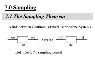
7.0 Sampling 7.1 The Sampling Theorem. A link between Continuous-time/Discrete-time Systems. Sampling. x [ n ]. y [ n ]. x ( t ). y ( t ). h [ n ]. h ( t ). x [ n ]= x ( nT ), T : sampling period. Sampling. Motivation: handling continuous-time signals/systems

E N D
7.0 Sampling • 7.1 The Sampling Theorem • A link between Continuous-time/Discrete-time Systems Sampling x[n] y[n] x(t) y(t) h[n] h(t) • x[n]=x(nT), T : sampling period
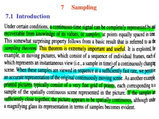
Motivation: handling continuous-time signals/systems • digitally using computing environment • accurate, programmable, flexible, • reproducible, powerful • compatible to digital networks and relevant • technologies • all signals look the same when digitized, • except at different rates, thus can be supported by a single network • Question: under what kind of conditions can a • continuous-time signal be uniquely specified by its discrete-time samples? • See Fig. 7.1, p.515 of text • Sampling Theorem
Impulse Train Sampling • See Fig. 7.2, p.516 of text • See Fig. 4.14, p.300 of text
Impulse Train Sampling • periodic spectrum, superposition of scaled, shifted replicas of X(jω) • See Fig. 7.3, p.517 of text
Impulse Train Sampling • Sampling Theorem (1/2) • x(t) uniquely specified by its samples x(nT), n=0,1, 2…… • precisely reconstructed by an ideal lowpass filter with Gain T and cutoff frequency ωM < ωc< ωs- ωM • applied on the impulse train of sample values • See Fig. 7.4, p.519 of text
Impulse Train Sampling • Sampling Theorem (2/2) • if ωs ≤ 2 ωM • spectrum overlapped, frequency components confused --- aliasing effect • can’t be reconstructed by lowpass filtering • See Fig. 7.3, p.518 of text
Impulse Train Sampling • Practical Issues • nonideal lowpass filters accurate enough for practical purposes determined by acceptable level of distortion • oversampling ωs = 2 ωM + ∆ ω • sampled by pulse train with other pulse shapes • signals practically not bandlimited : pre-filtering
Sampling with A Zero-order Hold • Zero-order Hold: • holding the sampled value until the next sample taken • modeled by an impulse train sampler followed by a system with rectangular impulse response
Sampling with A Zero-order Hold • Reconstructed by a lowpass filter Hr(jω) • See Fig. 7.6, 7.7, 7.8, p.521, 522 of text
Interpolation • Impulse train sampling/ideal lowpass filtering • See Fig. 7.10, p.524 of text
Interpolation • Zero-order hold can be viewed as a “coarse” interpolation • See Fig. 7.11, p.524 of text • Sometimes additional lowpass filtering naturally applied • e.g. viewed at a distance by human eyes, mosaic • smoothed naturally • See Fig. 7.12, p.525 of text
Interpolation • Higher order holds • zero-order : output discontinuous • first-order : output continuous, discontinuous • derivatives • See Fig. 7.13, p.526, 527 of text • second-order : continuous up to first derivative • discontinuous second derivative
Aliasing • Consider a signal x(t)=cos ω0t • sampled at sampling frequency • reconstructed by an ideal lowpass filter • with • xr(t) : reconstructed signal • fixed ωs, varying ω0
Aliasing • Consider a signal x(t)=cos ω0t • when aliasing occurs, the original frequency ω0 takes on the identity of a lower frequency, ωs – ω0 • w0 confused with not only ωs + ω0, but ωs – ω0 • See Fig. 7.15, 7.16, p.529-531 of text
Aliasing • Consider a signal x(t)=cos ω0t • many xr(t) exist such that • the question is to choose the right one • if x(t) = cos(ω0t + ϕ) • the impulses have extra phases ejϕ, e-jϕ
Aliasing • Consider a signal x(t)=cos ω0t • (a) (b) (c) (d) • phase also changed
Examples • Example 7.1, p.532 of text • (Problem 7.39, p.571 of text) sampled and low-pass filtered