Sampling Theorem
Sampling Theorem. 主講者:虞台文. Content. Periodic Sampling Sampling of Band-Limited Signals Aliasing --- Nyquist rate CFT vs. DFT Reconstruction of Band-limited Signals Discrete-Time Processing of Continuous-Time Signals Continuous-Time Processing of Discrete-Time Signals

Sampling Theorem
E N D
Presentation Transcript
Sampling Theorem 主講者:虞台文
Content • Periodic Sampling • Sampling of Band-Limited Signals • Aliasing --- Nyquist rate • CFT vs. DFT • Reconstruction of Band-limited Signals • Discrete-Time Processing of Continuous-Time Signals • Continuous-Time Processing of Discrete-Time Signals • Changing Sampling Rate • Realistic Model for Digital Processing
Sampling Theorem Periodic Sampling
C/D T Continuous to Discrete-Time Signal Converter xc(t) x(n)= xc(nT) Sampling rate
s(t) Conversion from impulse train to discrete-time sequence xs(t) x(n)= xc(nT) xc(t) C/D System
xc(t) xc(t) t t T 2T 3T 2T 0 T 2T 3T 4T 8T 4T 0 2T 4T 8T 10T x(n) x(n) n n 1 2 3 2 0 1 2 3 4 6 4 0 2 4 6 8 Sampling with Periodic Impulse train
xc(t) xc(t) t t T 2T 3T 2T 0 T 2T 3T 4T 8T 4T 0 2T 4T 8T 10T x(n) x(n) n n 1 2 3 2 0 1 2 3 4 6 4 0 2 4 6 8 We want to restore xc(t) from x(n). Sampling with Periodic Impulse train What condition has to be placed on the sampling rate?
s(t) Conversion from impulse train to discrete-time sequence xs(t) x(n)= xc(nT) xc(t) C/D System
s(t) Conversion from impulse train to discrete-time sequence xs(t) x(n)= xc(nT) xc(t) C/D System
C/D System s: Sampling Frequency
Sampling Theorem Sampling of Band-Limited Signals
Xc(j) 1 N N Yc(j) Band-Limited Signals Band-Limited Band-Unlimited
Xc(j) 1 N N 2/T S(j) s s 2s 2s 3s 3s S(j) 2/T 2s 2s 6s 4s 4s 6s Sampling of Band-Limited Signals Band-Limited Sampling with Higher Frequency Sampling with Lower Frequency
Sampling Theorem Aliasing --- Nyquist Rate
Xc(j) Band-Limited 1 N N Sampling with Higher Frequency 2/T S(j) s s 2s 2s 3s 3s Sampling with Lower Frequency S(j) 2/T 2s 2s 6s 4s 4s 6s Recoverability s > 2N s < 2N
Xc(j) 1 N N 2/T S(j) s s 2s 2s 3s 3s Xs(j) s s 2s 2s 3s 3s Case 1: s > 2N 1/T
Xc(j) 1 N N 2/T S(j) s s 2s 2s 3s 3s Xs(j) 1/T s s 2s 2s 3s 3s Case 1: s > 2N Passing Xs(j) through a low-pass filter with cutoff frequency N < c< s N , the original signal can be recovered. Xs(j) is a periodic function with period s.
Xc(j) 1 N N S(j) 2/T 2s 2s 4s 4s 6s 6s Xs(j) 2s 2s 4s 4s 6s 6s Case 2: s < 2N 1/T
Xc(j) 1 N N S(j) 2/T 2s 2s 4s 4s 6s 6s Xs(j) 1/T 2s 2s 4s 4s 6s 6s Case 2: s < 2N Xs(j) is a periodic function with period s. No way to recover the original signal. Aliasing
Xc(j) 1 N N Nequist Rate Band-Limited Nequist frequency (N) The highest frequency of a band-limited signal Nequist rate = 2N
Xc(j) 1 Band-Limited N N Nequist Sampling Theorem s > 2N Recoverable s < 2N Aliasing
Sampling Theorem CFT vs. DFT
s(t) Conversion from impulse train to discrete-time sequence xs(t) x(n)= xc(nT) xc(t) C/D System
s(t) Conversion from impulse train to discrete-time sequence xs(t) x(n)= xc(nT) xc(t) Continuous-Time Fourier Transform
s(t) Conversion from impulse train to discrete-time sequence xs(t) x(n)= xc(nT) xc(t) CFT vs. DFT x(n)
s(t) Conversion from impulse train to discrete-time sequence xs(t) x(n)= xc(nT) xc(t) x(n) CFT vs. DFT
Xc(j) 1 Xs(j) 1/T s s X(ej) 1/T 4 2 2 4 CFT vs. DFT
Xc(j) 1 Xs(j) 1/T s s X(ej) 1/T 4 2 2 4 CFT vs. DFT Amplitude scaling & Repeating Frequency scaling s2
Sampling Theorem Reconstruction of Band-limited Signals
xc(t) Xc(j) t T 3T 2T 0 T 2T 3T 4T /T /T X(ej) x(n) n 1 3 2 0 1 2 3 4 Key Concepts CFT ICFT Sampling C/D Retrieve One period FT IFT
Interpolation n(t) x(n)
Covert from sequence to impulse train Ideal Reconstruction Filter Hr(j) xr(t) xs(t) x(n) T T Ideal D/C Reconstruction System
Covert from sequence to impulse train Ideal Reconstruction Filter Hr(j) xr(t) xs(t) x(n) T T Hr(j) T /T /T Obtained from sampling xc(t) using an ideal C/D system. Ideal D/C Reconstruction System
Covert from sequence to impulse train Ideal Reconstruction Filter Hr(j) xr(t) xs(t) x(n) T T Ideal D/C Reconstruction System
xc(t) x(n) xr(t) C/D D/C T T Ideal D/C Reconstruction System In what condition xr(t) = xc(t)?
Sampling Theorem Discrete-Time Processing of Continuous-Time Signals
xc(t) x(n) y(n) yr(t) C/D D/C T T Continuous-Time System xc(t) yr(t) The Model Discrete-Time System
xc(t) yr(t) C/D Discrete-Time System D/C x(n) y(n) T T Continuous-Time System xc(t) yr(t) The Model H(ej) Heff(j)
xc(t) yr(t) C/D Discrete-Time System D/C x(n) y(n) H(ej) T T LTI Discrete-Time Systems Hr (j)
xc(t) yr(t) C/D Discrete-Time System D/C x(n) y(n) H(ej) Hr (j) T T LTI Discrete-Time Systems
Continuous-Time System xc(t) yr(t) LTI Discrete-Time Systems Heff(j)
xc(t) yr(t) C/D Discrete-Time System D/C H(ej) x(n) y(n) 1 T T c c Example:Ideal Lowpass Filter
Heff(j) 1 c c Continuous-Time System xc(t) yr(t) Example:Ideal Lowpass Filter
Continuous-Time System xc(t) Example: Ideal Bandlimited Differentiator
|Heff(j)| Continuous-Time System xc(t) Example: Ideal Bandlimited Differentiator
|Heff(j)| Continuous-Time System xc(t) Example: Ideal Bandlimited Differentiator
yc(t) Continuous-Time LTI system hc(t), Hc(j) D/C xc(t) yc(t) T Discrete-Time LTI System h(n) H(ej) xc(t) x(n) y(n) C/D T Impulse Invariance What is the relation between hc(t) and h(n)?