Download
1 / 13
140 likes | 546 Vues
Part II – TIME SERIES ANALYSIS C2 Simple Time Series Methods & Moving Averages. © Angel A. Juan & Carles Serrat - UPC 2007/2008. 2.2.1: Simple TS and Smoothing Methods.

E N D
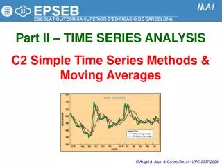
Part II – TIME SERIES ANALYSIS C2 Simple Time Series Methods & Moving Averages © Angel A. Juan & Carles Serrat - UPC 2007/2008
2.2.1: Simple TS and Smoothing Methods • The simple forecasting and smoothing methods model components in a series that are usually easy to see in a time series plot of the data. • These methods decompose the data into its trend and seasonal components, and then extend the estimates of the components into the future to provide forecasts. • Static methods have patterns that do not change over time; dynamic methods have patterns that do change over time and estimates are updated using neighboring values. • You may use two methods in combination. That is, you may choose a static method to model one component and a dynamic method to model another component. The decomposition approach to TSA involves an attempt to identify the component factors (Trend, Cyclical, Seasonal and Irregular) that influence each of the values in a series. Each component is identified separately. Projections of each of the components can then be combined to produce forecasts of future values of the time series. Naive methods are used to develop simple models that assume that very recent data provide the best predictors of the future. Averaging methods generate forecasts based on an average of past observations. Smoothing methods produce forecasts by averaging past values of a series with a decreasing (exponential) series of weights. • STATIC (SIMPLE) METHODS • Trend Analysis • Decomposition • DYNAMIC (SMOOTHING) METHODS • Moving Averages • Single Exponential Smoothing • Double Exponential Smoothing • Winters’ Method (Triple Exp. Smoothing) A disadvantage of combining methods is that the confidence intervals for forecasts are not valid.
2.2.2: Smoothing • If the time series data contain considerable error, smoothing is the first step in the process of trend identification. • It always involves some form of local averaging of data such that the nonsystematic components of individual observations cancel each other out. • The most common technique is Moving Averages (MA) smoothing which replaces each element of the series by either the simple or weighted average of m surrounding elements. • Medians can be used instead of means (results are then less biased by outliers) The MA method smooth out the “noise” in a time series. You have to select the MAlength, m. Different lengths provide different results.
2.2.3: Selecting a Simple Method or MA TREND ANALYSIS Series with trend but without seasonal component. It is often convenient to fit a trend curve to a time series for two reasons: (1) It provides some indication of the general direction of the observed series, and (2) it can be removed from the original series to get a clearer picture of the seasonality. CLASSICAL DECOMPOSITION Series with trend and seasonal component. The basic idea is to first estimate and remove the trend from the original series and then smooth out the irregular component. This leaves data containing only seasonal variation. The seasonal values are collected and summarized to produce a number (generally an index number) for each observed interval of the year. After the seasonal component has been isolated, it can be used to calculate seasonally adjusted data. MOVING AVERAGES (SMOOTHING) Series without trend and without seasonal component. A moving average of order k is the mean value of k consecutive observations. The most recent moving average value provides a forecast for the next period.
2.2.4: Measures of Accuracy Mean Absolute Percentage Error MAPE Mean Absolute Deviation MAD Mean Squared Deviation MSD One major difference between MSD and MAD is that the MSD measure is influenced much more by large fitting errors than by small errors (since for the MSD measure the errors are squared).
2.2.5: Moving Average Smoothing (1/2) To smooth the unpredictable ups and downs of a time series, you can form averages of consecutive observations. A strategy frequently used by some stock market investors is to buy if the current price of the stock exceeds the average of its ten most recent prices. Conversely, if the present price is lower than the average of the last ten, it is time to sell.
2.2.5: Moving Average Smoothing (2/2) • File: RIVERC.MTW • Stat > Time Series > Moving Average… Different lengths provide different results. You can generate forecasts of future values of the series. Three measures of the accuracy of the fitted values are provided: Mean Squared Deviation (MSD), Mean Absolute Deviation (MAD), and Mean Absolute Percentage Error (MAPE).
2.2.6: Trend Analysis (2/2) • File: RIVERC.MTW • Stat > Time Series > Trend Analysis… Trend analysis is closely related to linear regression. You choose from among four models (Linear, Quadratic, Exponential and S-Curve) to fit a particular type of trend line to a time series. Use residuals to detrend the time series. You can generate forecasts of future values of the series. Three measures of the accuracy of the fitted values are provided: Mean Squared Deviation (MSD), Mean Absolute Deviation (MAD), and Mean Absolute Percentage Error (MAPE).
2.2.7: Seasonality • Seasonality is defined as an autocorrelation of order k, i.e., a correlation between each element i of the series and the element i-k; k is called the lag. • If the measurement error is not too large, seasonality can be visually identified in the series as a pattern that repeats every k elements. A model that treats the time-series values as a sum of the components is called an additive components model: Yt = Tt + St + It A model that threats the time-series values as the product of the components is called a multiplicative components model: Yt = Tt * St * It Seasonal components can be additive in nature or multiplicative. For example, during the month of December the sales for a particular toy may increase by 1 million dollars every year. Thus, we could add to our forecasts for every December the amount of 1 million dollars (over the respective annual average) to account for this seasonal fluctuation. In this case, the seasonality is additive. Alternatively, during the month of December the sales for a particular toy may increase by 40%, that is, increase by a factor of 1.4. in this case the seasonal component is multiplicative in nature. In plots of the series, the distinguishing characteristic between these two types of seasonal components is that in the additive case, the series shows steady seasonal fluctuations, regardless of the overall level of the series; in the multiplicative case, the size of the seasonal fluctuations vary, depending on the overall level of the series.
2.2.8: Classical Decomposition (2/3) • File: RIVERC.MTW • Stat > Time Series > Decomposition… Classical decomposition separates the time series into trend, seasonal and error components by using least-squares analysis, trend analysis, and moving averages. You can select either a multiplicative or an additive model. In this case, an additive model with a seasonal length of 24 hours has been chosen. Initial fits overestimate actual values, indicating that a problem may exist. The graph depicts a slight download trend, with a 24-hour seasonal component. It also reflects the divergence of the predicted values from the actual values at the top of peaks and at the last valley. This window includes plots of the original data, detrended data, seasonally adjusted data, and the seasonally adjusted and detrended data. Note the unusual pattern at the end of the last two time series plots.
2.2.8: Classical Decomposition (3/3) • File: RIVERC.MTW • Stat > Time Series > Decomposition… This window provides a seasonal analysis for the time series data. It contains a plot of the seasonal indices. In addition, by seasonal period, it contains plots of the original data, present variation, and residuals. Some of these concepts will be explained in detail in future chapters. Note the large number of negative residuals present in four of the five last periods in the Residuals plot.