Data Analytics
Data Analytics. (Sub j ect C o de: 4 1 0 243 ) (Class: BE Co m p u ter E ngineeri n g) 2 0 1 5 P attern Designed By: Prof Vishakha Bhadane. Institute Vision "Satisfy the aspirations of youth force, who want to lead nation towards prosperity through techno-economic development."

Data Analytics
E N D
Presentation Transcript
Data Analytics (SubjectCode:410243) (Class:BEComputerEngineering) 2015Pattern Designed By: Prof VishakhaBhadane
Institute Vision "Satisfy the aspirations of youth force, who want to lead nation towards prosperity through techno-economic development." Institute Mission To provide, nurture and maintain an environment of high academic excellence, research & entrepreneurship for all aspiring students, which will prepare them to face global challenges maintaining high ethical and moral standards." Department Vision Empowering the students to be professionally competent & socially responsible for techno-economic development of society. Department Mission • To provide quality education enabling students for higher studies, research & entrepreneurship • To inculcate professionalism and ethical values through day to day practices.
Objectives andoutcomes CourseObjectives • – – – – Tounderstandandapplydifferentdesignmethodsandtechniques Tounderstandarchitecturaldesignandmodeling Tounderstandandapplytestingtechniques To implement design and testing using current tools and techniquesindistributed,concurrentandparallel Environments – • CourseOutcomes – – Topresentasurveyondesigntechniquesforsoftwaresystem TopresentadesignandmodelusingUMLforagivensoftware system Topresentadesignoftestcasesandimplementautomatedtesting forclientserver,distributed,mobileapplications – 2
OtherInformation • TeachingSchemeLectures: –3Hrs/Week ExaminationScheme • – – InSemesterAssessment:30 EndSemesterAssessment:70 3
Concepts UNIT-II Basic Data Analytic Methods 4
UNIT-I CONCEPTS Syllabus Statistical Methods for Evaluation- Hypothesis testing, difference of means, wilcoxon rank–sum test, type 1 type 2 errors, power and sample size, ANNOVA. Advanced Analytical Theory and Methods: Clustering- Overview, K means- Use cases, Overview of methods, determining number of clusters, diagnostics, reasons to choose and cautions. 4
3.3 Statistical Methods for EvaluationSubsections • 3.3.1 Hypothesis Testing • 3.3.2 Difference of Means • 3.3.3 Wilcoxon Rank-Sum Test • 3.3.4 Type I and Type II Errors • 3.3.5 Power and Sample Size • 3.3.6 ANOVA (Analysis of Variance)
3.3.1 Hypothesis Testing • Basic concept is to form an assertion and test it with data • Common assumption is that there is no difference between samples (default assumption) • Statisticians refer to this as the null hypothesis (H0) • The alternative hypothesis (HA) is that there is a difference between samples
3.3.1 Hypothesis TestingExample Null and Alternative Hypotheses
3.3.2 Difference of MeansTwo populations – same or different?
3.3.2 Difference of MeansTwo Parametric Methods • Student’s t-test • Assumes two normally distributed populations, and that they have equal variance • Welch’s t-test • Assumes two normally distributed populations, and they don’t necessarily have equal variance
3.3.3 Wilcoxon Rank-Sum TestA Nonparametric Method • Makes no assumptions about the underlying probability distributions
3.3.4 Type I and Type II Errors • An hypothesis test may result in two types of errors • Type I error – rejection of the null hypothesis when the null hypothesis is TRUE • Type II error – acceptance of the null hypothesis when the null hypothesis is FALSE
3.3.5 Power and Sample Size • The power of a test is the probability of correctly rejecting the null hypothesis • The power of a test increases as the sample size increases • Effect size d= difference between the means • It is important to consider an appropriate effect size for the problem at hand
3.3.6 ANOVA (Analysis of Variance) • A generalization of the hypothesis testing of the difference of two population means • Good for analyzing more than two populations • ANOVA tests if any of the population means differ from the other population means
4.1 Overview of Clustering • Clustering is the use of unsupervised techniques for grouping similar objects • Supervised methods use labeled objects • Unsupervised methods use unlabeled objects • Clustering looks for hidden structure in the data, similarities based on attributes • Often used for exploratory analysis • No predictions are made
4.2 K-means Algorithm • Given a collection of objects each with n measurable attributes and a chosen value k of the number of clusters, the algorithm identifies the k clusters of objects based on the objects proximity to the centers of the k groups. • The algorithm is iterative with the centers adjusted to the mean of each cluster’s n-dimensional vector of attributes
4.2.1 Use Cases • Clustering is often used as a lead-in to classification, where labels are applied to the identified clusters • Some applications • Image processing • With security images, successive frames are examined for change • Medical • Patients can be grouped to identify naturally occurring clusters • Customer segmentation • Marketing and sales groups identify customers having similar behaviors and spending patterns
4.2.2 Overview of the MethodFour Steps • Choose the value of k and the initial guesses for the centroids • Compute the distance from each data point to each centroid, and assign each point to the closest centroid • Compute the centroid of each newly defined cluster from step 2 • Repeat steps 2 and 3 until the algorithm converges (no changes occur)
4.2.2 Overview of the MethodExample – Step 1 Set k = 3 and initial clusters centers
4.2.2 Overview of the MethodExample – Step 2 Points are assigned to the closest centroid
4.2.2 Overview of the MethodExample – Step 3 Compute centroids of the new clusters
4.2.2 Overview of the MethodExample – Step 4 • Repeat steps 2 and 3 until convergence • Convergence occurs when the centroids do not change or when the centroids oscillate back and forth • This can occur when one or more points have equal distances from the centroid centers • Videos • http://www.youtube.com/watch?v=aiJ8II94qck • https://class.coursera.org/ml-003/lecture/78
4.2.3 Determining Number of Clusters • Reasonable guess • Predefined requirement • Use heuristic – e.g., Within Sum of Squares (WSS) • WSS metric is the sum of the squares of the distances between each data point and the closest centroid • The process of identifying the appropriate value of k is referred to as finding the “elbow” of the WSS curve
4.2.3 Determining Number of ClustersExample of WSS vs #Clusters curve The elbow of the curve appears to occur at k = 3.
4.2.3 Determining Number of ClustersHigh School Student Cluster Analysis
4.2.4 Diagnostics • When the number of clusters is small, plotting the data helps refine the choice of k • The following questions should be considered • Are the clusters well separated from each other? • Do any of the clusters have only a few points • Do any of the centroids appear to be too close to each other?
4.2.4 DiagnosticsSix clusters from points of previous figure
4.2.5 Reasons to Choose and Cautions • Decisions the practitioner must make • What object attributes should be included in the analysis? • What unit of measure should be used for each attribute? • Do the attributes need to be rescaled? • What other considerations might apply?
4.2.5 Reasons to Choose and CautionsObject Attributes • Important to understand what attributes will be known at the time a new object is assigned to a cluster • E.g., customer satisfaction may be available for modeling but not available for potential customers • Best to reduce number of attributes when possible • Too many attributes minimize the impact of key variables • Identify highly correlated attributes for reduction • Combine several attributes into one: e.g., debt/asset ratio
4.2.5 Reasons to Choose and CautionsObject attributes: scatterplot matrix for seven attributes
4.2.5 Reasons to Choose and CautionsUnits of Measure • K-means algorithm will identify different clusters depending on the units of measure k = 2
4.2.5 Reasons to Choose and CautionsUnits of Measure Age dominates k = 2
4.2.5 Reasons to Choose and CautionsRescaling • Rescaling can reduce domination effect • E.g., divide each variable by the appropriate standard deviation Rescaled attributes k = 2
4.2.5 Reasons to Choose and CautionsAdditional Considerations • K-means sensitive to starting seeds • Important to rerun with several seeds – R has the nstart option • Could explore distance metrics other than Euclidean • E.g., Manhattan, Mahalanobis, etc. • K-means is easily applied to numeric data and does not work well with nominal attributes • E.g., color