Download

1 / 23
230 likes | 358 Vues
Study of response uniformity of LHCb ECAL. Mikhail Prokudin, ITEP. Outline. Motivation Geometry of modules Experimental setup Procedure MC modeling Results light yield Conclusion. “Shashlik” technology cheap fast enough trigger radiation hard easy to segment Resolution

E N D
Study of response uniformity of LHCb ECAL Mikhail Prokudin, ITEP
Outline • Motivation • Geometry of modules • Experimental setup • Procedure • MC modeling • Results • light yield • Conclusion
“Shashlik” technology cheap fast enough trigger radiation hard easy to segment Resolution a – stochastic term~8%/sqrt(E) b – constant term stochasticterm decrease thickness of absorber increased volume ratio increased Morier radius more shower overlaps keep volume ratioconstant photostatistics constant term increase the volume ratio technology die-mold price ~10k $ MC model of light propagation in scintillator tile Motivation RD36 data 7%
Modules geometry • LHCb • inner: 4x4cm2 cells • middle: 6x6cm2 cells • outer: 12x12cm2 cells • 67x4mm layers of scintillator • 66x2mmlayers of lead • Prototype • 4x4cm2 cells • 280x0.5mm layers of scintillator • 280x0.5mm layers of lead
Calorimeter Experimental setup old chambers new chamber Beam Beam plug e, μ 25.111m 10.97m 2.935 LED monitoring system scheme Calorimeter assembly LED2 8 modules (12x12cm2x1) for leakage control PIN LED1 testing module
Coordinate determination • Beam size: 3x3cm2 • Energy cut: 60-65% MPV position • Details of calorimeter construction are visible Muons Shifts corrected for each position Same procedure for electrons
Muons. Procedure • energy only in central cell • 1x1 mm2 regions • fit with Landau distribution • first fit to estimate ranges • second fit with • f(xstart)=0.4*Max • f(xend)=0.05*Max • no Landau Gauss convolution • much more statistics
Electrons. procedure • Collect energy in 3x3+4 cells • wider signals with if other 4 cells included • 1x1 mm2 regions • Iterative fit procedure • [-1.2δ, +2δ] region
MC modeling • Signal nonuniformity • Light collection nonuniformity • Special ray tracer program • Scintillator tile thickness variations • Measured directly • Convolution with particle energy deposition • “natural” smearing • energy deposition nonuniformity • dead material • GEANT
Optics refraction Fresnel formulas reflection mirror diffuse attenuation in medium on surface all processes could depend on wavelength Geometry geometrical primitives cylinder box Boolean operations voxelization Main optical parameters quality of scintillator surface whiteness of paint size of “edging” Ray tracer program
Example of ray tracer test • Edge effect in light collection • compensate dead material between tiles • not trivial • LHCb innovation
LHCb inner module Muons Electrons Scale!
LHCb inner module. Muons Electrons Between fibers Between fibers Near fibers Near fibers Gray – MC. Black – data. Scale!
Prototype module Prototype. 0.5мм LHCb. 4мм Scale!
Prototype module and inner LHCb module LHCb inner Prototype Between fibers Between fibers Near fibers Near fibers Gray – MC. Black – data. Scale!
LHCb outer module • 12x12cm2 • Distance between fibers 15mm • 10mm in inner module • Only 2 delay wire chambers • worse position resolution • One set of optical parameters to describe all data! Between fibers Near fibers Gray – MC. Black – data.
Light yield Experiment • Use monitoring system MC • Generate photons uniformly inside tile volume • Inner module for normalization
Measurements of uniformity of LHCb calorimeter response presented different probes electrons muons different modules inner outer prototype absorber and scintillator thickness 0.5mm Calorimeter response uniformity modeled thickness measurements light collection ray tracer code developed tile model created Geant dead material simulation Model parameters extracted and checked for various geometries Conclusions
Coordinate determination • Modify coefficients • residuals • keep mean at 0 • narrow • Cut χ2<4 • denominator from “Delay wire chambers...” by J.Spanggaard.
Ray tracer testing • Visualize trajectories • individual photons • using ROOT for drawing
Geant model Steel tape, 0.2 mm • Geant3 • Gorynych framework • for ITEP FLINT experiment • Tile model with holes and fibers • same as for ray-tracing • 67x4mm scintillator layers • 66x2mm layers of lead • Dead material • steel tape, 0.2mm thick • white paint, 0.15mm at edge of tile White paint, 0.15 mm Fiber in each hole