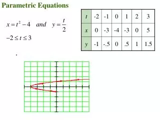
Parametric Equations
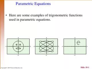
Parametric Equations. Here are some examples of trigonometric functions used in parametric equations. INTRODUCTION. Imagine that a particle moves along the curve C shown here. It is impossible to describe C by an equation of the form y = f ( x ).

Parametric Equations
E N D
Presentation Transcript
Parametric Equations • Here are some examples of trigonometric functions used in parametric equations.
INTRODUCTION • Imagine that a particle moves along the curve C shown here. • It is impossible to describe C by an equation of the form y = f(x). • This is because C fails the Vertical Line Test.
INTRODUCTION • However, the x- and y-coordinates of the particle are functions of time. So, we can write x = f(t) and y = g(t).
INTRODUCTION • Such a pair of equations is often a convenient way of describing a curve and gives rise to the following definition.
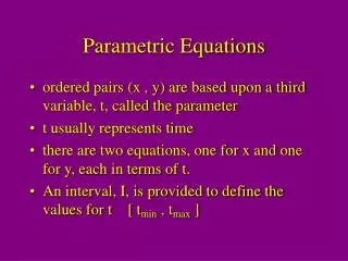
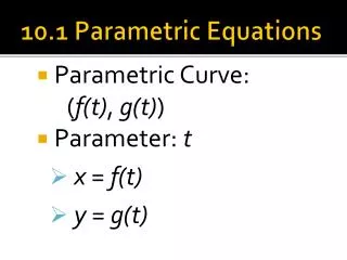
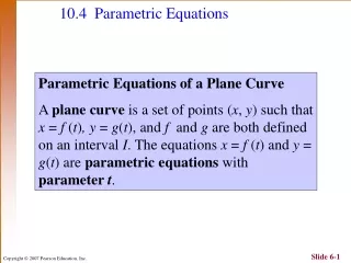
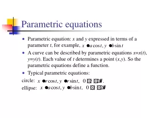
PARAMETRIC EQUATIONS • Suppose x and y are both given as functions of a third variable t (called a parameter) by the equations x = f(t) and y = g(t) • These are called parametric equations.
PARAMETRIC CURVE • Each value of t determines a point (x, y),which we can plot in a coordinate plane. • As t varies, the point (x, y) = (f(t), g(t)) varies and traces out a curve C. • This is called a parametric curve.
PARAMETER t • The parameter t does not necessarily represent time.
PARAMETER t • However, in many applications of parametric curves, t does denote time. • Thus, we can interpret (x, y) = (f(t), g(t)) as the position of a particle at time t.
10.7 Graphing a Circle with Parametric Equations Example Graph x = 2 cos t and y = 2 sin t for 0 2. Find an equivalent equation using rectangular coordinates. Solution Let X1T = 2 cos (T) and Y1T = 2 sin (T), and graph these parametric equations as shown. Technology Note Be sure the calculator is set in parametric mode. A square window is necessary for the curve to appear circular.
10.7 Graphing a Circle with Parametric Equations To verify that this is a circle, consider the following. The parametric equations are equivalent to x2 + y2 = 4, which is a circle with center (0, 0) and radius 2. x = 2 cos t, y = 2sin t cos2t + sin2t = 1
10.7 Graphing an Ellipse with Parametric Equations Example Graph the plane curve defined by x = 2 sin t and y = 3 cos t for t in [0, 2]. Solution Now add both sides of the equation.
10.7 Graphing a Cycloid • The path traced by a fixed point on the circumference of a circle rolling along a line is called a cycloid. A cycloid is defined by x = at – a sin t, y = a – a cos t, for t in (–, ) where a is the diameter. Example Graph the cycloid with a = 1 for t in [0, 2]. Analytic Solution There is no simple way to find a rectangular equation for the cycloid from its parametric equation.
10.7 Graphing a Cycloid Find a table of values and plot the ordered pairs.
10.7 Graphing a Cycloid Graphing Calculator Solution • Interesting Physical Property of the Cycloid If a flexible wire goes through points P and Q, and a bead slides due to gravity without friction along this path, the path that requires the shortest time takes the shape of an inverted cycloid.
10.7 Applications of Parametric Equations • Parametric equations are used frequently in computer graphics to design a variety of figures and letters. Example Graph a “smiley” face using parametric equations. Solution Head Use the circle centered at the origin. If the radius is 2, then let x = 2 cos t and y = 2 sin t for 0 t 2.
10.7 Applications of Parametric Equations Eyes Use two small circles. The eye in the first quadrant can be modeled by x = 1 + .3 cos t and y = 1 + .3 sin t. This represents a circle centered at (1, 1) with radius .3. The eye in quadrant II can be modeled by x = –1 + .3 cos t and y = 1 + .3 sin t for 0 t 2, which is a circle centered at (–1, 1) with radius 0.3. Mouth Use the lower half of a circle. Try x = .5 cos ½t and y = –.5 –.5 sin ½t. This is a semicircle centered at (0, –.5) with radius .5. Since t is in [0, 2], the term ½t ensures that only half the circle will be drawn.
10.7 Simulating Motion with Parametric Equations • If a ball is thrown with a velocity v feet per second at an angle with the horizontal, its flight can be modeled by the parametric equations where t is in seconds and h is the ball’s initial height above the ground. The term –16t2 occurs because gravity pulls the ball downward. Figure 80 pg 10-128
10.7 Simulating Motion with Parametric Equations Example Three golf balls are hit simultaneously into the air at 132 feet per second making angles of 30º, 50º, and 70º with the horizontal. • Assuming the ground is level, determine graphically which ball travels the farthest. Estimate this distance. • Which ball reaches the greatest height? Estimate this height. Solution (a) The three sets of parametric equations with h = 0 are as follows. X1T = 132 cos (30º) T, Y1T = 132 sin (30º) T – 16T2 X2T = 132 cos (50º) T, Y2T = 132 sin (50º) T – 16T2 X3T = 132 cos (70º) T, Y3T = 132 sin (70º) T – 16T2
10.7 Simulating Motion with Parametric Equations With 0 t 9, a graphing calculator in simultaneous mode shows all three balls in flight at the same time. The ball hit at 50º goes the farthest at an approximate distance of 540 feet. • The ball hit at 70º reaches the greatest height of about 240 feet.
10.7 Examining Parametric Equations of Flight Example A small rocket is launched from a table that is 3.36 feet above the ground. Its initial velocity is 64 feet per second, and it is launched at an angle of 30º with respect to the ground. Find the rectangular equation that models this path. What type of path does the rocket follow? Solution Its path is defined by the parametric equations x = (64 cos 30º)t and y = (64 sin 30º)t – 16t2 + 3.36 or, equivalently, From we get
10.7 Examining Parametric Equations of Flight Substituting into the other parametric equation yields The rocket follows a parabolic path.
10.7 Analyzing the Path of a Projectile Example Determine the total flight time and the horizontal distance traveled by the rocket in the previous example. Solution The equation y = –16t2 + 32t + 3.36 tells the vertical position of the rocket at time t. Find t for which y = 0 since this corresponds to the rocket at ground level. Since t represents time, t = –.1 is an unacceptable answer. Therefore, the flight time is 2.1 seconds. Use t = 2.1 to find the horizontal distance x as follows.
Homework Pages 584 – 585 1 – 5, 8 -11