Download
1 / 35
350 likes | 469 Vues
This wrap-up discusses critical concepts from previous lectures on network topologies and metabolic networks. Topics include a review of Barabasi & Oltvai's contribution to understanding metabolic networks, emphasizing properties like scale-free topology and clustering coefficients. The structural analysis of the Saccharomyces cerevisiae protein-interaction network illustrates how hubs maintain network integrity. Additionally, the significance of degree distribution and scale-free network properties is highlighted, emphasizing their implications for biological systems. Prepare for Q&A sessions about the lectures and assignments scheduled for February.

E N D
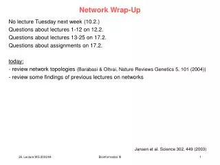
Network Wrap-Up • No lecture Tuesday next week (10.2.) • Questions about lectures 1-12 on 12.2. • Questions about lectures 13-25 on 17.2. • Questions about assignments on 17.2. • today: • review network topologies (Barabasi & Oltvai, Nature Reviews Genetics 5, 101 (2004)) • review some findings of previous lectures on networks Jansen et al. Science 302, 449 (2003) Bioinformatics III
Characterising metabolic networks To study the network characteristics of the metabolism a graph theoretic description needs to be established. (a) Here, the graph theoretic description for a simple pathway (catalysed by Mg2+-dependant enzymes) is illustrated. (b) In the most abstract approach all interacting metabolites are considered equally. The links between nodes represent reactions that interconvert one substrate into another. For many biological applications it is useful to ignore co-factors, such as the high-energy-phosphate donor ATP, which results (c) in a second type of mapping that connects only the main source metabolites to the main products. Barabasi & Oltvai, Nature Reviews Genetics 5, 101 (2004) Bioinformatics III
Characterising metabolic networks (d) The degree distribution, P(k) of the metabolic network illustrates its scale-free topology. (e) The scaling of the clustering coefficient C(k) with the degree k illustrates the hierarchical architecture of metabolism (The data shown in d and e represent an average over 43 organisms). (f) The flux distribution in the central metabolism of Escherichia coli follows a power law, which indicates that most reactions have small metabolic flux, whereas a few reactions, with high fluxes, carry most of the metabolic activity. It should be noted that on all three plots the axis is logarithmic and a straight line on such log–log plots indicates a power-law scaling. CTP, cytidine triphosphate; GLC, aldo-hexose glucose; UDP, uridine diphosphate; UMP, uridine monophosphate; UTP, uridine triphosphate. Barabasi & Oltvai, Nature Reviews Genetics 5, 101 (2004) Bioinformatics III
Yeast protein interaction network A map of protein–protein interactions in Saccharomyces cerevisiae, which is based on early yeast two-hybrid measurements, illustrates that a few highly connected nodes (which are also known as hubs) hold the network together. The largest cluster, which contains 78% of all proteins, is shown. The colour of a node indicates the phenotypic effect of removing the corresponding protein (red = lethal, green = non-lethal, orange = slow growth, yellow = unknown). Barabasi & Oltvai, Nature Reviews Genetics 5, 101 (2004) Bioinformatics III
Degree The most elementary characteristic of a node is its degree (or connectivity), k, which tells us how many links the node has to other nodes. For example, in the undirected network shown in part a of the figure, node A has degree k = 5. In networks in which each link has a selected direction (see figure, part b) there is an incoming degree, kin, which denotes the number of links that point to a node, and an outgoing degree, kout, which denotes the number of links that start from it. For example, node A in part b of the figure has kin = 4 and kout = 1. An undirected network with N nodes and L links is characterized by an average degree <k> = 2L/N (where <> denotes the average). Barabasi & Oltvai, Nature Reviews Genetics 5, 101 (2004) Bioinformatics III
Degree distribution The degree distribution, P(k), gives the probability that a selected node has exactly k links. P(k) is obtained by counting the number o f nodes N(k) with k = 1,2... links and dividing by the total number of nodes N. The degree distribution allows us to distinguish between different classes of networks. For example, a peaked degree distribution, as seen in a random network, indicates that the system has a characteristic degree and that there are no highly connected nodes (which are also known as hubs). By contrast, a power-law degree distribution indicates that a few hubs hold together numerous small nodes. Barabasi & Oltvai, Nature Reviews Genetics 5, 101 (2004) Bioinformatics III
Network measures Scale-free networks and the degree exponent Most biological networks are scale-free, which means that their degree distribution approximates a power law, P(k) k-, where is the degree exponent and ~ indicates 'proportional to'. The value of determines many properties of the system. The smaller the value of , the more important the role of the hubs is in the network. Whereas for >3 the hubs are not relevant, for 2> >3 there is a hierarchy of hubs, with the most connected hub being in contact with a small fraction of all nodes, and for = 2 a hub-and-spoke network emerges, with the largest hub being in contact with a large fraction of all nodes. In general, the unusual properties of scale-free networks are valid only for < 3, when the dispersion of the P(k) distribution, which is defined as 2 = <k2> - <k>2, increases with the number of nodes (that is, diverges), resulting in a series of unexpected features, such as a high degree of robustness against accidental node failures. For >3, however, most unusual features are absent, and in many respects the scale-free network behaves like a random one. Barabasi & Oltvai, Nature Reviews Genetics 5, 101 (2004) Bioinformatics III
Shortest path and mean path length Distance in networks is measured with the path length, which tells us how many links we need to pass through to travel between two nodes. As there are many alternative paths between two nodes, the shortest path — the path with the smallest number of links between the selected nodes — has a special role. In directed networks, the distance ℓAB from node A to node B is often different from the distance ℓBA from B to A. For example, in part b of the figure, ℓBA = 1, whereas ℓAB = 3. Often there is no direct path between two nodes. As shown in part b of the figure, although there is a path from C to A, there is no path from A to C. The mean path length, <ℓ>, represents the average over the shortest paths between all pairs of nodes and offers a measure of a network's overall navigability. Barabasi & Oltvai, Nature Reviews Genetics 5, 101 (2004) Bioinformatics III
Clustering coefficient In many networks, if node A is connected to B, and B is connected to C, then it is highly probable that A also has a direct link to C. This phenomenon can be quantified using the clustering coefficient33CI = 2nI/k(k-1), where nI is the number of links connecting the kI neighbours of node I to each other. In other words, CI gives the number of 'triangles' that go through node I, whereas kI (kI -1)/2 is the total number of triangles that could pass through node I, should all of node I's neighbours be connected to each other. For example, only one pair of node A's five neighbours in part a of the figure are linked together (B and C), which gives nA = 1 and CA = 2/20. By contrast, none of node F's neighbours link to each other, giving CF = 0. The average clustering coefficient, <C >, characterizes the overall tendency of nodes to form clusters or groups. An important measure of the network's structure is the function C(k), which is defined as the average clustering coefficient of all nodes with k links. For many real networks C(k) k-1, which is an indication of a network's hierarchical character. The average degree <k>, average path length <ℓ> and average clustering coefficient <C> depend on the number of nodes and links (N and L) in the network. By contrast, the P(k) and C(k ) functions are independent of the network's size and they therefore capture a network's generic features, which allows them to be used to classify various networks. Barabasi & Oltvai, Nature Reviews Genetics 5, 101 (2004) Bioinformatics III
Origin of scale-free topology and hubs in biological networks The origin of the scale-free topology in complex networks can be reduced to two basic mechanisms: growth and preferential attachment. Growth means that the network emerges through the subsequent addition of new nodes, such as the new red node that is added to the network that is shown in part a . Preferential attachment means that new nodes prefer to link to more connected nodes. For example, the probability that the red node will connect to node 1 is twice as large as connecting to node 2, as the degree of node 1 (k1=4) is twice the degree of node 2 (k2 =2). Growth and preferential attachment generate hubs through a 'rich-gets-richer' mechanism: the more connected a node is, the more likely it is that new nodes will link to it, which allows the highly connected nodes to acquire new links faster than their less connected peers. In protein interaction networks, scale-free topology seems to have its origin in gene duplication. Part b shows a small protein interaction network (blue) and the genes that encode the proteins (green). When cells divide, occasionally one or several genes are copied twice into the offspring's genome (illustrated by the green and red circles). This induces growth in the protein interaction network because now we have an extra gene that encodes a new protein (red circle). The new protein has the same structure as the old one, so they both interact with the same proteins. Ultimately, the proteins that interacted with the original duplicated protein will each gain a new interaction to the new protein. Therefore proteins with a large number of interactions tend to gain links more often, as it is more likely that they interact with the protein that has been duplicated. This is a mechanism that generates preferential attachment in cellular networks. Indeed, in the example that is shown in part b it does not matter which gene is duplicated, the most connected central protein (hub) gains one interaction. In contrast, the square, which has only one link, gains a new link only if the hub is duplicated. Barabasi & Oltvai, Nature Reviews Genetics 5, 101 (2004) Bioinformatics III
Random networks Aa The Erdös–Rényi (ER) model of a random network starts with N nodes and connects each pair of nodes with probability p, which creates a graph with approximately pN (N-1)/2 randomly placed links. Ab The node degrees follow a Poisson distribution, which indicates that most nodes have approximately the same number of links (close to the average degree <k>). The tail (high k region) of the degree distribution P(k ) decreases exponentially, which indicates that nodes that significantly deviate from the average are extremely rare. Ac The clustering coefficient is independent of a node's degree, so C(k) appears as a horizontal line if plotted as a function of k. The mean path length is proportional to the logarithm of the network size, l log N, which indicates that it is characterized by the small-world property. Barabasi & Oltvai, Nature Reviews Genetics 5, 101 (2004) Bioinformatics III
Scale-free networks Scale-free networks are characterized by a power-law degree distribution; the probability that a node has k links follows P(k) ~ k- , where is the degree exponent. The probability that a node is highly connected is statistically more significant than in a random graph, the network's properties often being determined by a relatively small number of highly connected nodes that are known as hubs (see figure, part Ba; blue nodes). In the Barabási–Albert model of a scale-free network, at each time point a node with M links is added to the network, which connects to an already existing node I with probability I = kI/JkJ, where kI is the degree of node I and J is the index denoting the sum over network nodes. The network that is generated by this growth process has a power-law degree distribution that is characterized by the degree exponent = 3. Bb Such distributions are seen as a straight line on a log–log plot. The network that is created by the Barabási–Albert model does not have an inherent modularity, so C(k) is independent of k (Bc). Scale-free networks with degree exponents 2< <3, a range that is observed in most biological and non-biological networks, are ultra-small, with the average path length following ℓ ~ log log N, which is significantly shorter than log N that characterizes random small-world networks. Barabasi & Oltvai, Nature Reviews Genetics 5, 101 (2004) Bioinformatics III
Hierarchical networks To account for the coexistence of modularity, local clustering and scale-free topology in many real systems it has to be assumed that clusters combine in an iterative manner, generating a hierarchical network. The starting point of this construction is a small cluster of four densely linked nodes (see the four central nodes in Ca). Next, three replicas of this module are generated and the three external nodes of the replicated clusters connected to the central node of the old cluster, which produces a large 16-node module. Three replicas of this 16-node module are then generated and the 16 peripheral nodes connected to the central node of the old module, which produces a new module of 64 nodes. The hierarchical network model seamlessly integrates a scale-free topology with an inherent modular structure by generating a network that has a power-law degree distribution with degree exponent = 1 + ln4/ln3 = 2.26 (see Cb) and a large, system-size independent average clustering coefficient <C> ~ 0.6. The most important signature of hierarchical modularity is the scaling of the clustering coefficient, which follows C(k) ~ k-1 a straight line of slope -1 on a log–log plot (see Cc). A hierarchical architecture implies that sparsely connected nodes are part of highly clustered areas, with communication between the different highly clustered neighbourhoods being maintained by a few hubs (see Ca). Barabasi & Oltvai, Nature Reviews Genetics 5, 101 (2004) Bioinformatics III
Reminder A few remarks on the past lectures ... Bioinformatics III
V14: Prediction of P-P interaction from correlated mutations Results obtained by i2h in a set of 14 two domain proteins of known structure = proteins with two interacting domains. Treat the 2 domains as different proteins. A: Interaction index for the 133 pairs with 11 or more sequences in common. The true positive hits are highlighted with filled squares. B: Representation of i2h results, reminiscent of those obtained in the experimental yeast two-hybrid system. The diameter of the black circles is proportional to the interaction index; true pairs are highlighted with gray squares. Empty spaces correspond to those cases in which the i2h system could not be applied, because they contained <11 sequences from different species in common for the two domains. In most cases, i2h scored the correct pair of protein domains above all other possible interactions. Pazos, Valencia, Proteins 47, 219 (2002) Bioinformatics III
V14: Co-localization of interaction partners Use localization data to assess the quality of prediction because two predicted interacting partners sharing the same subcellular location are more likely to form a true interaction. Comparison of colocalization index (defined as the ratio of the number of protein pairs in which both partners have the same subcellular localization to the number of protein pairs where both partners have any sub-cellular localization annotation). Multithreading predictions (MTA) are less reliable than high-confidence inter-actions, but score quite well amongst predictions + HTS screens. Lu, ..., Skolnick, Genome Res 13, 1146 (2003) Bioinformatics III
V14:Do partners have the same function? Proteins from different groups of biological functions may interact with each other. However, the degree to which interacting proteins are annotated to the same functional category is a measure of quality for predicted interactions. Here, the predictions cluster fairly well along the diagonal. Lu, ..., Skolnick, Genome Res 13, 1146 (2003) Bioinformatics III
V15: Statistical significance of complexes and modules Number of complete cliques (Q = 1) as a function of clique size enumerated in the network of protein interactions (red) and in randomly rewired graphs (blue, averaged >1,000 graphs where number of interactions for each protein is preserved). Inset shows the same plot in log-normal scale. Note the dramatic enrichment in the number of cliques in the protein-interaction graph compared with the random graphs. Most of these cliques are parts of bigger complexes and modules. Spirin, Mirny, PNAS 100, 12123 (2003) Bioinformatics III
V15: Architecture of protein network Fragment of the protein network. Nodes and interactions in discovered clusters are shown in bold. Nodes are colored by functional categories in MIPS: red, transcription regulation; blue, cell-cycle/cell-fate control; green, RNA processing; and yellow, protein transport. Complexes shown are the SAGA/TFIID complex (red), the anaphase-promoting complex (blue), and the TRAPP complex (yellow). Spirin, Mirny, PNAS 100, 12123 (2003) Bioinformatics III
V15: Evolution of the yeast protein interaction network Isotemporal categories are designed through a binary (b) coding scheme. The b code represents the distribution of each yeast protein's orthologs in the universal tree of life. Bit value 1 indicates the presence of at least one orthologous hit for a yeast protein in a corresponding group of genomes, and bit value 0 indicates the absence of any orthologous hit. The presented example is 110011 in the b format and 51 in the d format. Orthologous identifications are based on COGs at NCBI and in von Mering et al. (2002). Previously, phylogenetic profiles were used to detect protein interaction partners. Here, use phylogenetic profiles to detect modules. Qin et al. PNAS 100, 12820 (2003) Bioinformatics III
V15: Evolution of the yeast protein interaction network Interaction patterns. Z scores for all possible interactions of the isotemporal categories in the protein interaction network. For categories i and j, Zi,j = (Fi,jobs – Fi,jmean)/i,j where Fi,jobs is the observed number of interactions, and Fi,jmean and i,j are the average number of interactions and the SD, respectively, in 10,000 MS02 null models. The diagonal distribution of large positive Z scores indicates that yeast proteins tend to interact with proteins from the same or closely related isotemperal categories. Qin et al. PNAS 100, 12820 (2003) Bioinformatics III
V19: Flux balancing mass conservation. Therefore one may analyze metabolic systems by requiring mass conservation. Only required: knowledge about stoichiometry of metabolic pathways and metabolic demands For each metabolite: Under steady-state conditions, the mass balance constraints in a metabolic network can be represented mathematically by the matrix equation: S· v = 0 where the matrix S is the m n stoichiometric matrix, m = the number of metabolites and n = the number of reactions in the network. The vector v represents all fluxes in the metabolic network, including the internal fluxes, transport fluxes and the growth flux. Any chemical reaction requires Bioinformatics III
V19: Flux balance analysis Since the number of metabolites is generally smaller than the number of reactions (m < n) the flux-balance equation is typically underdetermined. Therefore there are generally multiple feasible flux distributions that satisfy the mass balance constraints. The set of solutions are confined to the nullspace of matrix S. To find the „true“ biological flux in cells ( e.g. Heinzle, Huber, UdS) one needs additional (experimental) information, or one may impose constraints on the magnitude of each individual metabolic flux. The intersection of the nullspace and the region defined by those linear inequalities defines a region in flux space = the feasible set of fluxes. Bioinformatics III
V19: Rerouting of metabolic fluxes (Black) Flux distribution for the wild-type. (Red) zwf- mutant. Biomass yield is 99% of wild-type result. (Blue) zwf- pnt- mutant. Biomass yield is 92% of wildtype result. The solid lines represent enzymes that are being used, with the corresponding flux value noted. Note how E.coli in silico circumvents removal of one critical reaction (red arrow) by increasing the flux through the alternative G6P P6P reaction. Edwards & Palsson PNAS 97, 5528 (2000) Bioinformatics III
V20: Extreme Pathways introduced into metabolic analysis by the lab of Bernard Palsson (Dept. of Bioengineering, UC San Diego). The publications of this lab are available at http://gcrg.ucsd.edu/publications/index.html Extreme pathway technique is based on the stoichiometric matrix representation of metabolic networks. All external fluxes are defined as pointing outwards. Schilling, Letscher, Palsson, J. theor. Biol. 203, 229 (2000) Bioinformatics III
V20: Feasible solution set for a metabolic reaction network (A) The steady-state operation of the metabolic network is restricted to the region within a cone, defined as the feasible set. The feasible set contains all flux vectors that satisfy the physicochemical constrains. Thus, the feasible set defines the capabilities of the metabolic network. All feasible metabolic flux distributions lie within the feasible set, and (B) in the limiting case, where all constraints on the metabolic network are known, such as the enzyme kinetics and gene regulation, the feasible set may be reduced to a single point. This single point must lie within the feasible set. Edwards & Palsson PNAS 97, 5528 (2000) Bioinformatics III
V21: Reconfigured Network A(ext) B(ext) C(ext) R1 R2 R3 R4 B R8 R7f R7b A C P R5 R9 R6 D 3 EFMs are not systemically independent: EFM1 = EP4 + EP5 EFM2 = EP3 + EP5 EFM4 = EP2 + EP3 Klamt & Stelling Trends Biotech 21, 64 (2003) Bioinformatics III
V21: relation between EP and EFMs What is the consequence of when all exchange fluxes (and hence all reactions in the network) are irreversible? EFMs and EPs always co-incide! Klamt & Stelling Trends Biotech 21, 64 (2003) Bioinformatics III
V22: Correlation between genes of same metabolic pathway Genes of the glycolysis pathway (according KEGG) were clustered and ordered based on the correlation in their expression profiles. Shown here is the matrix of their pair-wise correlations. The cluster of highly correlated genes (orange frame) corresponds to genes that encode the central glycolysis enzymes. The linear arrangement of these genes along the pathway is shown at right. Of the 46 genes assigned to the glycolysis pathway in the KEGG database, only 24 show a correlated expression pattern. In general, the coregulated genes belong to the central pieces of pathways. Ihmels, Levy, Barkai, Nat. Biotech 22, 86 (2004) Bioinformatics III
V22: Connectivity of metabolites The connectivity of a given metabolite is defined as the number of reactions connecting it to other metabolites. Shown are the distributions of connectivity between metabolites in an unrestricted network () and in a network where only correlated reactions are considered (). In accordance with previous results (Jeong et al. 2000) , the connectivity distribution between metabolites follows a power law (log-log plot). In contrast, when coexpression is used as a criterion to distinguish functional links, the connectivity distribution becomes exponential (log-linear plot). Ihmels, Levy, Barkai, Nat. Biotech 22, 86 (2004) Bioinformatics III
V22: Co-expression of transporters Transporter genes are co-expressed with the relevant metabolic pathways providing the pathways with its metabolites. Co-expression is marked in green. Ihmels, Levy, Barkai, Nat. Biotech 22, 86 (2004) Bioinformatics III
V25: Combination of data sets into probabilistic interactomes The 4 interaction data sets from HT experiments were combined into 1 PIE. The PIE represents a transformation of the individual binary-valued interaction sets into a data set where every protein pair is weighed according to the likelihood that it exists in a complex. (B) Combination of data sets into probabilistic interactomes. A „naïve” Bayesian network is used to model the PIP data. These information sets hardly overlap. Because the 4 experimental interaction data sets contain correlated evidence, a fully connected Bayesian network is used. Jansen et al. Science 302, 449 (2003) Bioinformatics III
V25: Static naive Bayesian Networks The likelihood ratio L defined as relates prior and posterior odds according to Bayes‘ rule: In the special case that the N features are conditionally independent (i.e. they provide uncorrelated evidence) the Bayesian network is a so-called „naïve” network, and L can be simplified to: Jansen et al. Science 302, 449 (2003) Bioinformatics III
V25: PIP vs. the information sources Ratio of true to false positives (TP/FP) increases monotonically with Lcut, confirming L as an appropriate measure of the odds of a real interaction. The ratio is computed as: Protein pairs with Lcut > 600 have a > 50% chance of being in the same complex. Jansen et al. Science 302, 449 (2003) Bioinformatics III
V25: PIE vs. the information sources 9897 interactions are predicted from PIP and 163 from PIE. In contrast, likelihood ratios derived from single genomic factors (e.g. mRNA coexpression) or from individual interaction experiments (e.g. the Ho data set) did no exceed the cutoff when used alone. This demonstrates that information sources that, taken alone, are only weak predictors of interactions can yield reliable predictions when combined. Jansen et al. Science 302, 449 (2003) Bioinformatics III