Global Budget of Atmospheric 14 CO 2

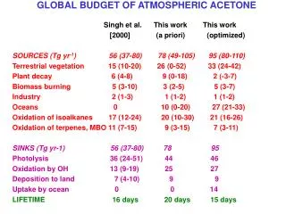
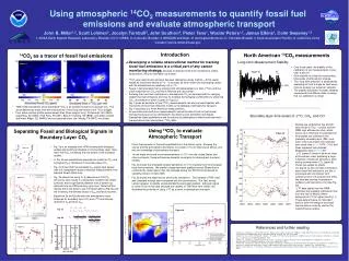
1. BNE NWR 1s = 2‰ 3 years A B C Biosphere disequilibrium Correction ~ <0.2 ppm Eq. 2a Eq. 2b Figure 3a Figure 2c D14CO2 (per mil; relative scale) 2004.0 2005.0 Using atmospheric 14CO2 measurements to quantify fossil fuel emissions and evaluate atmospheric transport John B. Miller1,2, Scott Lehman3, Jocelyn Turnbull3, John Southon4, Pieter Tans1, Wouter Peters1,2, James Elkins1, Colm Sweeney1,2 1. NOAA Earth System Research Laboratory, Boulder, CO 2. CIRES, U. Colorado, Boulder 3. INSTAAR and Dept. of Geological Sciences, U. Colorado Boulder 4. Keck Accelerator Facility, U. California, Irvine Contact: john.b.miller@noaa.gov Introduction North American 14CO2 measurements 14CO2 as a tracer of fossil fuel emissions •  Developing a reliable observational method for tracking fossil fuel emissions is a critical part of any carbon monitoring strategy,because inventories need to be verified and, unlike observations, they are inevitably out of date. • 14CO2 is an ideal fossil fuel tracer because radioactive decay (half life = 5700 years) leaves all fossil fuels devoid of 14C. In contrast, all other reservoirs exchanging carbon with the atmosphere are relatively rich in 14C. • Figure 1 demonstrates this by showing that simulated patterns of total D14CO2 and the fossil component of CO2 over North America are very similar. • Knowing the fossil fuel contribution to atmospheric CO2 is important both for verifying stated fossil fuel emissions and also for isolating the biological contributions to observed CO2, an example of which is given in Figure 2. • Fig. 3 gives an example of how 14CO2 measurements can also be used together with inventories of fossil fuel emissions to test our knowledge of atmospheric transport. • Fig. 4 describes our North American measurements. • As we make more and more measurements, we will be able to test not just model transport accuracy but our atmospheric top-down source estimation techniques themselves (data assimilations and inversions) by attempting to directly estimate fossil fuel emissions from atmospheric 14CO2 data. Long-term Measurement Stability Figure 1 • Over three years, the stability of the calibration of our measurements is very high: 2 per mil. • Such stability is critical for constructing time series of atmospheric change. • This ‘long-term precision’ is assessed by analyzing air from a single air tank every time we analyze our actual air samples. • The stability calculation includes samples measured at two different labs, showing that our calibration is robust. Figure 4a HFM Global Budget of Atmospheric 14CO2 • TM5 model simulations show that total Δ14CO2 is an excellent tracer for fossil fuel CO2.The small differences result from the contributions of non-fossil fuel terms to the 14CO2 budget. • Four active vertical profile measurement sites (three heights only): Portsmouth, NH (NHA), Cape May, NJ (CMA), Park Falls, WI (LEF), Beaver Crossing, NE (BNE); one active surface site Niwot Ridge, CO (NWR); and one planned tower site, Moody, TX (WKT) are shown. Boundary-layer time series of D14C, CO2, and CO • Sample are collected at five aircraft sites shown in Fig 1. (circles) and the NWR high altitude site (line), which serves as a reference of unpolluted air. • All samples are collected in the planetary boundary layer (PBL) and warm colors represent more polluted east coast sites (NHA, HFM, CMA) and blues represent less polluted Midwestern sites (BNE, LEF) • D14C (panel A) tends to be much lower at the eastern sites, indicating a large influence of fossil fuel emissions, even during summer when CO2 (panel B) shows net uptake by plants. • CO (panel C) also contains information about fossil fuel emissions, but this is convolved with information from numerous other CO sources and sinks, like biomass burning, hydrocarbon oxidation and removal by OH (see Fig. 2d). • D14C data higher than the NWR reference line probably indicate air flow from the Gulf of Mexico where background D14C is higher (see Fig. 1). • These data will allow for important tests of both the transport and fossil fuel emissions currently used in the CarbonTracker system. Using 14CO2 to evaluate Atmospheric Transport Separating Fossil and Biological Signals in Boundary Layer CO2 Figure 4b • Fossil fuel emission is the best quantified flux in the carbon cycle. Knowing the source and the atmospheric distribution of a tracer (D14C)for that source allows us to test our knowledge of atmospheric transport. • As we make more and more measurements of D14C over the United States and other continents, these will become powerful constraints for atmospheric transport models. • Fig. 3a shows the simulated surface distribution of D14C resulting from the European fossil fuel emissions. We predict a large east-west gradient across Siberia that is confirmed by observations (Fig. 3b) sampled during the TROICA-8 rail-based air sampling mission in April 2004. • Fig. 3b shows the observations and model simulations. Two variants of TM5 (‘fast’ and ‘standard’ mixing) were compared with the observations. The ‘fast’ mixing version appears to slightly underestimate the east-west gradient. Although signal-to-noise is low in this case because the variants of TM5 were very similar, this illustrates the potential of using D14C as a tracer of atmospheric transport. • Fig. 2a is an example from HFM showing both biological uptake and fossil fuel influence in the boundary layer. Here, fossil fuel CO2 is masking the true extent of the biological uptake. • In Fig. 2b we quantitatively separate the fossil fuel (Cff) and biological (Cbio) influences on boundary layer CO2. • Fig. 2c shows that the calculated Cbio signal (red) agrees well with independent eddy-covariance measurements from Harvard Forest (black line). • Fig. 2d shows that using Cff to determine a CO:CO2 emissions ratio results in a seasonally variable ratio (black symbols) that is significantly different from a bottom-up estimate from an EPA inventory (gray line). Note that this implies that if one were to use CO observations (Fig 2a) and the inventory, the derived values of Cbio would be incorrect. • Equations 2a and 2b describe the atmospheric mass balances for boundary layer CO2 and D14C and how we determine Cff and thus Cbio. Figure 2a Figure 2b Figure 3b References and further reading Figure 2d • Turnbull, J.C., J.B. Miller, S.J. Lehman, P.P. Tans, R.J. Sparks, and J. Southon, Comparison of (CO2)-C-14, CO, and SF6 as tracers for recently added fossil fuel CO2 in the atmosphere and implications for biological CO2 exchange, Geophys. Res. Lett., 33 (1), 2006. • Turnbull, J.C., S.J. Lehman, J.B. Miller,R. J. Sparks, J. R. Southon, P. P. Tans, A new high precision 14CO2 time series for North American continental air, J. Geophys. Res., 112, D11310, doi:10.1029/2006JD008184., 2007. • Turnbull, J.C., J.B. Miller, S.J. Lehman, W. Peters, P. P. Tans, J. Southon, D. Hurst, S. Montzka, J. Elkins Spatial distribution of D14CO2 across Eurasia: Measurements from the TROICA-8 expedition, In Prep for J. Geophys. Res., 2007. • Helliker, B.R., J.A. Berry, A.K. Betts, P.S. Bakwin, K.J. Davis, A.S. Denning, J.R. Ehleringer, J.B. Miller, M.P. Butler, and D.M. Ricciuto, Estimates of net CO2 flux by application of equilibrium boundary layer concepts to CO2 and water vapor measurements from a tall tower, J. Geophys. Res., 109 (D20), 2004. • Bakwin, P.S., K.J. Davis, C. Yi, S.C. Wofsy, J.W. Munger, L. Haszpra, and Z. Barcza Regional carbon dioxide fluxes from mixing ratio data, Tellus B, 56 (4), 301-311, 2004