Estimation CH8 Least Squares
Estimation CH8 Least Squares. 2011/08/6 劉永富. CH8 Least Square : 8.1 Introduction. Advantage NO probabilistic assumptions are made about the data, only a signal model is assumed. Easy to implement. Disadvantage NO claims about optimality can be made.

Estimation CH8 Least Squares
E N D
Presentation Transcript
EstimationCH8 Least Squares 2011/08/6 劉永富
CH8 Least Square : 8.1 Introduction • Advantage • NO probabilistic assumptions are made about the data, only a signal model is assumed. • Easy to implement. • Disadvantage • NO claims about optimality can be made. • The statistical performance cannot be assessed without some specific assumptions about the probabilistic structure of the data.
8.3 The Least Square Approach • In the Least Square (LS) approach, we attempt to minimize the squared difference between the given data x[n] and the assumed signal or noiseless data.
The least squares estimator (LSE) chooses the value that makes s[n] closest to the observed data x[n]. Closeness is measured by the LS error criterion • The value of that minimizes is the LSE. • Note that, NO probabilistic assumptions have been made about the data x[n].
The method is equally valid for Gaussian as well as non-Gaussian noise. • The performance of the LSE will undoubtedly depend upon the properties of the corrupting noise as well as any modeling errors. • LSEs are usually applied in situations where a precise statistical characterization of the data is unknown or where an optimal estimator cannot be found or may be too complicated to apply in practice.
Example 8.1 • Assume that the signal model in Fig. 8.1 is s[n]=A and we observe x[n] for n=0,1,…,N-1. By LS approach • Differentiating with respect to A and setting the result equal to zero • Our estimator, cannot be claimed to be optimal in the MVU sense but only in that it minimizes the LS error.
If , where w[n] is zero mean WGN, then the LSE will also be the MVU estimator, but otherwise not. • Suppose the noise is not zero mean • The observed data are composed of a deterministic signal and zero mean noise. • This modeling error would also cause the LSE to be biased.
Example 8.2 • Consider the signal model • The LSE is found by minimizing • The problem is a nonlinear least squares problem. • Nonlinear LS problems are solved via grid searches or iterative minimization methods as described in section 8.9.
Example 8.3 • Consider the signal model , where f0 is known and A is to be estimated. Then the LSE minimizes • This is easily accomplished by differentiation since J(A) is quadratic in A. • If A were known and the frequency were to be estimated, the problem would be equivalent to that in example 8.2.
In the vector parameter case, both A and f0 might need to be estimated. Then, the error criterion is quadratic in A but non-quadratic in f0. • J can be minimized in closed form with respect to A for a given f0, reducing the minimization of J to one overf0 only. • This type of problem is termed a separable least squares problem, which will discussed in section 8.9.
8.4 Linear Least squares • In applying the linear LS approach for a scalar parameter we must assume that where is a known sequence. • The LS error criterion becomes
8.4 Linear Least squares • For Example 8.1 and Original Reduction due to signal fitting
8.4 Linear Least squares • • If the data is noiseless (x[n] = A) Jmin = 0 • If The minimum LS error would then be
Extension • S: p x 1 H: N x p θ:p x 1 • The H is referred to as the observation matrix (P.84).
Compare with Ch 4 and Ch 6 • Setting the gradient equal to zero yields the LSE • For it to be the BLUE would require and , and to be efficient would in addition to these properties require x to be Gaussian. • Ch 6 :
Jmin Idempotent A2 = A
8.5 Geometrical interpretations • Recall the general signal model . If we denote the columns of H by hi, we have
Example 8.4 – Fourier Analysis • Referring to Example 4.2 (P.88), we suppose the signal model to be
Example 8.4 – Fourier Analysis • The LS error was defined to be
Example 8.5 (p.89) ∵ • And also
Example 8.5 • Therefore,
8.6 Order-Recursive Least Square • In many cases the signal model is unknown and must be assumed. Ex.
8.6 Order-Recursive Least Square • The following models might be assumed • Using a LSE with would produce the estimate for the intercept and slope as
8.6 Order-Recursive Least Square and • We plotted and where T=100.
8.6 Order-Recursive Least Square • The fit using two parameter is better, as expect. We will later show that the minimum LS error must decrease as we add more parameters. • The data are subject to error, we may very well be fitting the noise.
8.6 Order-Recursive Least Square • In practice, we increase the order of the polynomial until the minimum LS error decrease only slightly as the order is increased.
8.6 Order-Recursive Least Square • In this example the signal was actually and the noise was WGN with Note that if A, B had been estimated perfectly, the minimum LS error: • When true order is reached, This is verified in Fig8.6 and increase our confidence in the chosen model.
8.7 Sequential least squares • LSE (vector form) : . • Assume we have determined the LSE based on . If we now observe , we can update (in time) without having to resolve the linear equations . • The procedure is termed Sequential Least Squares.
Sequential least squares • Consider example 8.1 in which the DC signal level is to be estimated. The LSE is • If we now observe the new data sample , then the LSE becomes
Sequential least squares • The new LSE is found by using the previous one and the new observation • The new estimate is equal to the old one plus a correctionterm • If the error is zero, then no correction takes place for that update.
Estimator • The estimate appears to be converging to the true value of . This is in agreement with the variance approaching zero.