Simulation
Simulation. Supplement B. Simulation. Simulation : The act of reproducing the behavior of a system using a model that describes the processes of the system.

Simulation
E N D
Presentation Transcript
Simulation Supplement B
Simulation • Simulation: The act of reproducing the behavior of a system using a model that describes the processes of the system. • Time Compression: The feature of simulations that allows them to obtain operating characteristic estimates in much less time than is required to gather the same operating data from a real system. • Monte Carlo simulation: A simulation process that uses random numbers to generate simulation events.
Specialty Steel Products Co.Example B.1 • Specialty Steel Products Company produces items such as machine tools, gears, automobile parts, and other specialty items in small quantities to customer order. • Demand is measured in machine hours. • Orders are translated into required machine-hours. • Management is concerned about capacity in the lathe department. • Assemble the data necessary to analyze the addition of one more lathe machine and operator.
Weekly Production Relative Requirements (hr) Frequency 200 0.05 250 0.06 300 0.17 350 0.05 400 0.30 450 0.15 500 0.06 550 0.14 600 0.02 Total 1.00 Specialty Steel Products Co.Example B.1 Historical records indicate that lathe department demand varies from week to week as follows:
Weekly Production Relative Requirements (hr) Frequency 200 0.05 250 0.06 300 0.17 350 0.05 400 0.30 450 0.15 500 0.06 550 0.14 600 0.02 Total 1.00 Specialty Steel Products Co.Example B.1 Average weekly production is determined by multiplying each production requirement by its frequency of occurrence. Average weekly production requirements = 200(0.05) + 250(0.06) + 300(0.17) + … + 600(0.02) = 400 hours
Weekly Production Relative Requirements (hr) Frequency 200 0.05 250 0.06 300 0.17 350 0.05 400 0.30 450 0.15 500 0.06 550 0.14 600 0.02 Total 1.00 Specialty Steel Products Co.Example B.1 Regular Relative Capacity (hr) Frequency 320 (8 machines) 0.30 360 (9 machines) 0.40 400 (10 machines) 0.30 The average number of operating machine-hours in a week is: 320(0.30) + 360(0.40) + 400(0.30) = 360 hours Average weekly production requirements = 400 hours
Regular Relative Capacity (hr) Frequency 320 (8 machines) 0.30 360 (9 machines) 0.40 400 (10 machines) 0.30 Weekly Production Relative Requirements (hr) Frequency 200 0.05 250 0.06 300 0.17 350 0.05 400 0.30 450 0.15 500 0.06 550 0.14 600 0.02 Total 1.00 Regular Relative Capacity (hr) Frequency 360 (9 machines) 0.30 400 (10 machines) 0.40 440 (11 machines) 0.30 © 2007 Pearson Education Specialty Steel Products Co. The average number of operating machine-hours in a week = 360 Hrs. Experience shows that with 11 machines, the distribution would be: Average weekly production requirements = 400 hours Example B.1
Specialty Steel Products Co.Assigning Random Numbers • Random numbers must now be assigned to represent the probability of each demand event. • Random Number: A number that has the same probability of being selected as any other number. • Since the probabilities for all demand events add up to 100 percent, we use random numbers between (and including) 00 and 99. • Within this range, a random number in the range of 0 to 4 has a 5% chance of selection. • We can use this to represent our first weekly demand of 200 which has a 5% probability.
Random numbers in the range of 0-4 have a 5% chance of occurrence. Random numbers in the range of 5-10 have a 6% chance of occurrence. Random numbers in the range of 11-27 have a 17% chance of occurrence. Random numbers in the range of 28-32 have a 5% chance of occurrence. Specialty Steel Products Co.Assigning Random Numbers Event Weekly Demand (hr) Probability 200 0.05 250 0.06 300 0.17 350 0.05 400 0.30 450 0.15 500 0.06 550 0.14 600 0.02
Event Existing Weekly Random Weekly Random Demand (hr) Probability Numbers Capacity (hr) Probability Numbers 200 0.05 00–04 320 0.30 00–29 250 0.06 05–10 360 0.40 30–69 300 0.17 11–27 400 0.30 70–99 350 0.05 28–32 400 0.30 33–62 450 0.15 63–77 500 0.06 78–83 550 0.14 84–97 600 0.02 98–99 Specialty Steel Products Co.Assigning Random Numbers If we randomly choose numbers in the range of 00-99 enough times, 5 percent of the time they will fall in the range of 00-04, 6% of the time they will fall in the range of 05-10, and so forth.
Specialty Steel Products Co.Model Formulation • Formulating a simulation model entails specifying the relationship among the variables. • Simulation models consist of decision variables, uncontrollable variables and dependent variables. • Decision variables: Variables that are controlled by the decision maker and will change from one run to the next as different events are simulated. • Uncontrollable variables are random events that the decision maker cannot control.
Specialty Steel Products Co.Example B.2 Simulating a particular capacity level • Using the Appendix 2 random number table, draw a random number from the first two rows of the table. Start with the first number in the first row, then go to the second number in the first row. • Find the random-number interval for production requirements associated with the random number. • Record the production hours (PROD) required for the current week. • Draw another random number from row three or four of the table. • Find the random-number interval for capacity (CAP) associated with the random number. • Record the capacity hours available for the current week.
Specialty Steel Products Co.Example B.2 Simulating a particular capacity level • If CAP > PROD, then IDLE HR = CAP – PROD • If CAP < PROD, then SHORT = PROD – CAP If SHORT < 100 then OVERTIME HR = SHORT and SUBCONTRACT HR = 0 If SHORT > 100 then OVERTIME HR = 100 and SUBCONTRACT HR = SHORT – 100 • Repeat steps 1 - 8 until you have simulated 20 weeks.
10 Machines Existing Demand Weekly Capacity Weekly Sub- Random Production Random Capacity Idle Overtime contract Week Number (hr) Number (hr) Hours Hours Hours 1 71 450 50 360 90 2 68 450 54 360 90 3 48 400 11 320 80 4 99 600 36 360 100 140 5 64 450 82 400 50 6 13 300 87 400 100 7 36 400 41 360 40 . . . . . . . . . . . . . . . . . . . . . . . . 20 37 400 19 320 80 Total 490 830 360 Weekly average 24.5 41.5 18.0 © 2007 Pearson Education Specialty Steel Products Co.20-week simulation
Comparison of 1000-week Simulations 10 Machines 11 Machines Idle hours 26.0 42.2 Overtime hours 48.3 34.2 Subcontract hours 18.4 8.7 Cost $1,851.50 $1,159.50 Specialty Steel Products Co.1000-week simulation A steady state occurs when the simulation is repeated over enough time that the average results for performance measures remain constant.
Monte Carlo SimulationApplication B.1 Famous Chamois Car Wash Car Arrival Distribution (time between arrivals) Famous Chamois is an automated car wash that advertises that your car can be finished in just 15 minutes. The time until the next car arrival is described by the following distribution.
Monte Carlo SimulationApplication B.1 • Famous Chamois Car Wash:Random Number Assignment • Assign a range of random numbers to each event so that the demand pattern can be simulated.
Monte Carlo Simulation Famous Chamois Car Wash: Simulation Simulate the operation for 3 hours, using the following random numbers, assuming that the service time is constant at 6, (:06) minutes per car.
Computer Simulation • The simulation for Specialty Steel Products demonstrated the basics of simulation. • However it only involved one step in the process, with two uncontrollable variables (weekly production requirements and three actual machine-hours available) and 20 time periods. • Simple simulation models with one or two uncontrollable variables can be developed using Excel, using its random number generator. • More sophisticated simulations can become time consuming and require a computer.
BestCar Auto Dealer Simulation Model • Below is a probability distribution for the number of cars sold weekly at BestCar (See Example B.3). • The selling price per car is $20,000. Design a simulation model that determines the probability distribution and mean of the weekly sales.
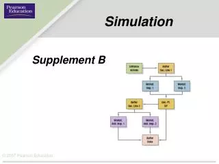
Simulation with SimQuick • Simquick is an easy-to-use package that is an Excel spreadsheet with some macros. • Let’s simulate the passenger security process at one terminal of a medium-sized airport between the hours of 8 A.M. and 10 A.M. • Passengers arrive in a single line and go through one of two inspection stations consisting of a metal detector and a carry-on baggage scanner. • After this, 10% are randomly selected for an additional inspection handled by one of two stations. • Management wants to examine the effects of increasing the number of random inspections to 15% and 20%. • They also want to consider a 3rd station for the 2nd inspection
Buffer Sec. Line 1 Work St. Insp. 1 Work St. Insp. 2 Buffer Sec. Line 2 Dec. Pt. DP Work St. Add. Insp. 1 Work St. Add. Insp. 2 Buffer Done Flowchart of Passenger Security Process Information about each block is entered into Simquick. Other information needed in statistical distribution form: (1) when people arrive, (2) inspection times, & (3) % of passengers randomly selected. Arrivals and inspection times are acquired through observation; % randomly selected is a policy decision Entrance Arrivals
Element Element Statistics Overall Types Names Means Entrance(s) Door Objects entering process 237.23 Buffer(s) Line 1 Mean inventory 5.97 Mean cycle time 3.12 Line 2 Mean inventory 0.10 Mean cycle time 0.53 Done Final inventory 224.57 Simulation Results of Passenger Security Process