Download
1 / 27
270 likes | 453 Vues
Visualizing Diffusion Tensor Dissimilarity using an ICA Based Perceptual Colour Metric. Mark S. Drew and Ghassan Hamarneh Vision and Media Lab Medical Image Analysis Lab Simon Fraser University {mark,hamarneh}@cs.sfu.ca. Diffusion tensor imaging.

E N D
Visualizing Diffusion Tensor Dissimilarity using an ICA Based Perceptual Colour Metric Mark S. Drew and Ghassan Hamarneh Vision and Media Lab Medical Image Analysis Lab Simon Fraser University {mark,hamarneh}@cs.sfu.ca
Diffusion tensor imaging • Diffusion “Tensor” — a 3 x 3 matrix at each voxel: xx, xy, xz, yx=xy, yy, yz, zx=xz, zy=yz, zz • Data is MR signal — enscapulates information on water diffusion, at the voxel. • Brownian motion, but tends to follows “tracts” ∴ can use to discover structure Best reference: Wandell, NIPS 2001 tutorial: Diffusion tensor imaging and fiber tractography of human brain pathways
Higher diffusion along tracts ⇛ = Complementary but different information from more traditional T1- and T2-weighted spin-echo MR data. ⇛ Useful for tasks such as inverse problem of locating epilepsy trigger locations from EEG values – use tensor values as electrical conductivity tensor in generalized Poisson equation.
xx, xy, xz, yx=xy, yy, yz, zx=xz, zy=yz, zz measurements in multiple directions So, 9 variables at each voxel, But symmetric, => 6 independent variables. Traditional visualization: use eigenvectors of each tensor.
Because tensor is diffusion, turns out that it’s positive semi-definite: diagonal Λ 0 (The diffusion at each sample location is represented by a 3x3 covariance.) D is symmetric => U is orthogonal, real.
The 3 columns of U are normalized 3-vectors, So typically visualize D by showing an ellipsoid, with axes along the eigenvectors, and lengths e.values. (or other glyphs, e.g. superquadrics)
What about colour? • Simple approaches have been used • and, little attention has been paid to forming colours that actually correspond to a difference metric within the structure being imaged! • Simply map the principal eigenvector at each pixel into {R,G,B} • colour the three components of the first eigenvector according to a pre-determined colour map • multiply the 3x3 matrix times a “probe vector”, and map to {R,G,B}; etc.
(i.e., Independent Component Analysis (see Drew and Bergner, CIC12, 2004 for a tutorial) • seems to extract main, noise-free diffusion signal as largest component; then other effects (eddy currents); then noise. So far, we looked at each voxel separately. => An approach to whole-brain analysis has been to compute ICA components
Can we map main signal to brightness, and modulate by assigning colour to other components? => That way, we code the main information into the visual channel with the most acuity, and reserve colour as a modulating factor encoding the remaining ICA information.
Can we map a meaningful metric into a perceptually meaningful metric in colour space? • The Log-Euclidean metric for DT data: • [Arsigny et al. MICCAI’05] • taking logs shown to provide reasonable metric • for differences between DTs at different voxels • but wish to maintain positive semi-definite property • so define “Log” function, via • Log(D) = U diag ( log ( diag ( ) ) ) UT
Want to go to 6-vector representation, for simplicity. But maintain same difference- measure as for 9 components:
So matrix F is the set of filters that corresponds to basis B: ICA on 6-vectors, for practical data, generates a rank-6 basis, B : i.e., B is 6x6. But B is not orthogonal, so must form pseudoinverse to find coefficients.
Diffusion Tensor Data and Perceptual Colour Consider brain scans (we’ll use 256x256x55 voxels, from http://lbam.med.jhmi.edu/) slice 25 T1-weighted DT: 1,1 component
DT is zero where there is no diffusion; so form 2D convex hull to use foreground DT signal: => v = vec(Log(D)) So coeff’s: c = F v => let’s look at coeff’s: 1 5 3 2 4 6
#1 all-positive since D is diagonally-dominant #1 most important (ordered by variance) sizes of these coefficients c :
So, algorithm proposed here: • map 6D perceptual color: L*, a*, b*: • ---------------------------------------------------- • map c1↦ L* ; • How to map remaining 5D into a*,b*? • Formv’ = (v – c1 b1), perform ICA again; • Repeat in remaining 4D space.
Now map L*, a*, b* to nonlinear sRGB display space: • L*, a*, b* ↦ XYZ tristimulus values (nonlinear transform) • XYZ ↦ sRGBlinear (linear, plus clipping) • sRGBlinear ↦sRGB (if-statement + gamma-correction)
Test on a synthetic phantom: ↦ (plus 5% Gaussian noise)
Some results: slice 5 slice 50 slice 24 slice 26 slice 25
55 slices: scalar T1 tensor DT tensor enhances perception of organization & connectivity
CC standard subdivision, ↦ tone curves for histogram equalization Test: can this really help in visualization? -- Consider Corpus Callosum segmentation: vertical slice (sagittal)
Compare to FA (histeq’d): FA previously used to distinguish the seven segments: Apply Tone curves to whole brain:
sRGB colour: F-statistic=32.5 At least one confidence interval does not overlap, from segment to segment – facilitating differentiating them. Which measure can best discriminate regions of distinct diffusion properties? 95% confidence intervals overlap: can’t differentiate segments. FA — F-statistic=29.9 log(D) — F-statistic=22.6
How do the 7 segments look in L*,a*,b*? CIELAB coordinates for the means in the seven CC segments (coloured using the mean sRGB colour from the histeq CC): substantial change in CIELAB between segments.
Future: … • ! Cleaner visualization : We'd like to segment, e.g. using extension of the Mean-Shift segmentation algorithm; • should allow for easier evaluation for diagnosis, by medical experts • ! Other methods of assigning CIELAB using distance-preserving dimensionality reduction: • We've used ICA = a linear method (as is PCA) • Non-linear mappings: • -- MDS Multidimensional Scaling for assigning location in a low-D space • -- LLE Locally Linear Embedding (based on proximity matrices via a graph); • -- Isomap - another graph-based method for nonlinear dimensionality reduction
Thanks! To Natural Sciences and Engineering Research Council of Canada