Download
1 / 45
450 likes | 623 Vues
Update on D 0 reconstruction using Vertex ing (TPC+ SSD+SVT). Secondary micro-vertexing methods Reports on tests performed with : Simulation : pure D 0 sample Simulation : mixed D 0 sample in AuAu hijing Real data summary. BNL : Y. Fisyak, V. Perevoztchikov

E N D
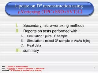
Update on D0 reconstruction using Vertexing(TPC+SSD+SVT) Secondary micro-vertexing methods Reports on tests performed with : Simulation : pure D0 sample Simulation : mixed D0 sample in AuAu hijing Real data summary BNL : Y. Fisyak, V. Perevoztchikov KSU : J. Bouchet, J. Joseph, S. Margetis, J. VanFossen Subatech : W. Borowski, A. Geromitsos, S. Kabana,
Fitting approaches for secondary vertices • GOAL : To know with precision the position of secondary vertex of decaying particle to apply topological cut. • Challenging for charmed particles because of the small c (for D0, c ~122 µm) • We are investigating 3-methods • A Linear Fit approach : three lines fit with errors (two tracks plus a parent from the event vertex). 2. A Helix swimming to DCA of the two track helices (V0-like) : a. using the global track parameters to reconstruct helices (StPhysicalHelix) of both tracks candidates. b. using the parameters from StDcaGeometry 3. A Full Helix Fitwith errors (a.k.a. TCFit) - it will allow momentum dependent cut using the full track information. All this work is directly applicable to HFT
We have reported a discrepancy when using the helix swimming (each panel shows the correlation of the 2nd vertex reconstructed vs 2nd vertex from GEANT, for pure D0),for the 3 methods (top to bottom) : an horizontal band, ie GEANT says that two tracks come from common point but helix swim finds large DCA at secondary vertex->not real minimum but something else. The linear fit method shows no correlation (abandoned) Linear fit global Position of decay vertex - GEANT DCAG X Y Z Reconstructed • it is understood now as daughter tracks decaying back-to-back : • http://cnr2.kent.edu/~vanfossen/MySTARPage/D0_uVertexing/Entries/2009/10/15_Pure_D0_secVtx_Reco_and_Phi.htmlc J. VanFossen
Low pT D0 (i) • The daughters are decaying back to back and the parallelism causes poor resolution • D0 momentum almost null for daughters ~ 18030 deg. • Want to exploit this correlation to find a possible D0 signal in low momentum. J. Joseph
Workshop@subatech • In december, there was a workshop in Nantes about the micro-vertexing techniques • Talks can be found here : • http://drupal.star.bnl.gov/STAR/blog/bouchet/2009/dec/21/micro-vertexing-workshop-subatech-15-17-dec-2009 • Work done by W. Borowski and A. Geromitsos : • http://www.star.bnl.gov/~borowski/evo/09-12-17 look on CuCu data (btag sample) for e-D0 correlation and evaluate , for the D0, it’s characteristics (decay length, dca between daughters) by doing selection based on S/B ,where S = pure D0 and B= real data
Evaluation of Full Fit (TCFIT) Strategy : Use pure D0 sample to find cuts and check that it works (3k events) Use mixed sample : 1 D0 embedded in Hijing event (10k events): Use y2007g geometry (last updated for AuAu in simu : http://drupal.star.bnl.gov/STAR/comp/prod/MCGeometry Follow these different steps : Produce AuAu MB 200GeV as background Produce 1 D0 per event Mix fz files from background and D0 Do the reconstruction with slow simulation for the TPC+ silicon detectors. Analyze MuDst.root file (it consists in reconstructed tracks), with same code used for real data analysis) 3. Look at the real data using cuts found in 1. and 2. *For step 1. and 2., D0 is forced (BR =100%) to decay in K-π+
A few words on the Full Helix Fit • TCFIT is a least square fit of the decay vertex, under constraints. [1] • In 2 bodies decay, combine 2 tracks under the constraint that they’re coming from a common point. • Add constraints (momentum conservation, mass hypothesis) to minimize of the 2 (The probability is the minimization of the 2of the fit [3]) • Code from [2] uses 1 constraint (decay length) and returns its value, probability and total 2. • In the next slides, I compared these results (TCFIT) with the helix swimming method and the input from GEANT. 2 =∑ (qi-h(x,pi))T V-1i (qi-h(x,pi)) tracks i Parametrisation of the track (helix) covariance matrix of measured track parameters measured track parameters [1]Decay Chain Fitting with a Kalman Filter,W. D. Hulsbergen http://arxiv.org/abs/physics/0503191 [2]$Star/StRoot/StarRoot/TCFit.cxx [3]http://en.wikipedia.org/wiki/Chi-square_distribution
A) Probability plots : pure D0 sample • For thepure D0 sample : • Expect flat distribution for pure D0 • Expect a peak at low probability and a decreasing curve for background • TCFIT (as implemented) uses 1 constraint fit : momentum conservation at decay vertex • Peak at probability <.01 still here for expected signal (red): • Underestimation of errors (errors of TCFIT ~ hits error + track error • When increasing the track errors, we observe the probability distribution gets an assymetry being more at large probability. : http://www.star.bnl.gov/~bouchet/TCFIT/covMatrix.htm • #entries(probability<10%) / all Entries • All : 35.5% • K-+ : 34.48% • K+- : 37.14% we choose to apply a cut at probability > .01 to remove the wrong topological decays calculated by TCFIT.
Signed decay length (TCFIT) vs decay length (THelix) Pure D0 sample Probability>0.01
Signed decay length (TCFIT) vs decay length (GEANT) rms mean rms mean • all the next plots have pT >1 • decay length from GEANT is the distance (in 3d) between the componants of the PV and the vertex associated to track with GEANT_ID = 37 (D0) Pure D0 sample No cut on the probability
Signed decay length (TCFIT) vs decay length (GEANT) rms mean rms mean Pure D0 sample Probability>0.01
Comments • we see : • a correlation between the decay length from TCFIT and the decay length calculated by the helix swimming. • a nice correlation between the decay length from TCFIT and the decay length in GEANT. • We reported previously (J. VanFossen) the correlation between the decay length calculated by the helix swimming and GEANT. • There is no systematic shift in reconstructed quantities (mean~0) and the resolution is about 250 microns, independent of pt (expected for SSD+SSD’s resolutions)
slength based cuts investigation All pair tracks Unlike sign Same sign Goal : use the results from TCFIT (decay length, its error and probability) to apply topological cuts [Jonathan what are the plots? Data, simulation?]
Subtraction:positive-negative L/dL contribution • For the K-+ case : • subtraction of # of entries bin to bin first positive bin entries are subtracted with first negative bin, and so on First negative bin First positive bin difference
B) Probability of TCFIT : mixed sample Number of tracks < 200 All pair tracks Unlike sign Same sign zoom Number of tracks < 200 All pair tracks Unlike sign Same sign • Same observation as the pure sample, peak at very low probability is observed • Next slide : explanation of the cut N < 200 tracks.
Invariant Mass plots • Check : plots w/o any cuts on decay length • nor probability of TCFIT • Fit of mass+background : • Linear + Breit-Wigner where the fit • function is : • a + bMreco + Γ/[(Mreco -MPDG)2 + (Γ/2)2 ] No cuts on N = number of primary tracks (per event) All the following plots are from mix D0 sample (SIMULATION) s/n ~12.3 N < 200 • We used the cut N < 200 based on previous observation where a clear signal appears • It would be easier to investigate the effects of other cuts if already a signal is present.
Unlike-like sign invariant mass plots N = number of primary tracks
Cut on low multiplicities We were using a cut (<200) on the number of primary track N to get a signal in simu/mix data. • The plot shows the number of primary tracks (per event) for real data : • we cut the ‘interesting’ part of the event where the S/sqrt(B) is higher as S scales with binary collisions and B as N2 so sqrt(B)~ # of participants • In simu we embed one D0 per event flat in pT so correlation with real data is complex 1 D0 per event 2000 tracks 0 need other cuts to remove/reduce the huge combinatoric background
Applying a positive cut L/dL >2 (only) no cut with The cut • When applying only the cut on L/dL, a peak at the invariant mass of the D0 is appearing • we can bypass the multiplicity cut
summary • Only positive cut has to be applied. • cuts like |L/dL| is not correct since it also selects slength < 0 • (=wrong topological decay fitting)
c) Real data-QA : Scan of DCA resolution - run 7 MinBias ,Production2 Issues Improvement for DCA resolution estimation : Dependence with η Dependence with particle Id Cuts |zvertex |<5 cm : to have a clean sample TPC hits> 15 || in SSD range (~ ||<1.2) pT >0.1 Fit function : Reflect the (detector+alignment) resolution and Multiple Coulomb Scattering Fit done for 0.2 < 1/P < 5 In the next plots, x-axis = day number (day 110 = April, 20th, day 170 = June,19th) DCA resolution@1GeV (for tracks with N=2,3,4) vs day number to study stability of DCA resolution. • 4(ssd+svt)3(svt only) silicon hits , pointing resolution ~ 220 m at P = 1GeV/c • The details are here : • Minbias per run: • http://drupal.star.bnl.gov/STAR/system/files/test_histo_MB_allDetails.pdf • Production2 per run : • http://drupal.star.bnl.gov/STAR/system/files/test_histo_P2_allDetails.pdf • Minbias, day110 : DCA resolution per eta-phi slices: • http://drupal.star.bnl.gov/STAR/system/files/Eta_Phi_histo_Allsilicon_noerrorsbar.pdf
Pointing resolution Pointing Resolution MinBias Production 2 Number of Tracks with 0,1,2,3,4 silicon hits • The idea is to use tracks with silicon hits (3 or 4) to reach enough DCA pointing resolution to make cuts based on DCA of daughters. (from the K-π+ association) • Stable during the run. • The more each track has silicon hits, the better the pointing resolution is. • But it represents a small fraction.
Real Data (production2) • Up to now (01/10) : ~ 500000 events 170000 events after vertex cuts The removal of the cut on the number of tracks will allow us to explore the full event (not only low multiplicities). • All combinations • after dEdx + momentum cuts • after inv. Mass window cut • after TCFIT cuts • This sample will be our working sample • for cut studies. Cuts applied directly in the code
slength /slength_error • The plots show the signed decay length divided by its error for all pair tracks (left) and pairs tracks requiring 3 or more silicon hits (right) as a function of the Kπ pair pT. • Note : we consider only the K-π+ combination. • L/dL has a flat distribution around L/dL ~ 2
Invariant mass vs L/dL cut (no silicon hit cut) • Need more statistic to see the effect of largeL/dL cut. • A cut based on the track • quality (ie its DCA/DCA) as well • may be needed to select only ‘good’ tracks.
Investigation of other cuts Negative values for D0 signal • In Andrea Dainese’s thesis[1], he used a combination of cuts based on the product of DCA of daughters to the primary vertex (PV) and the angle formed by the D0 momentum and the vector joining the PV and secondary vertex. [1] :arXiv:nucl-ex/0311004
For the pure sample signal : K-π+ background : K+π- signal : K-π+ background : K+π-
Summary/ next steps • TCFIT : the full helix fit with errors (cov. matrix of tracks) is implemented, tested and used now. • Yuri Fisyak will work on an improvement because this method uses numerical derivations that take time & CPU. • More relevant since now we don’t apply the cut on the multiplicity = large number of tracks associations. • Previous issues are understood as low pT D0 : work is ongoing to take advantage of these particular decay. • Simulation : a comparison of TCFIT results with helix swimming and GEANT are in agreement • In parallel of real data reproduction, we investigate some precise cuts • Real data : • Tracks with N>1 benefit from the SVT points precision : the DCA resolution vs time is stable for these cases. • Need statistic now !
DcaGeometry Pt_GL (first hit) . (circle center) Pt @ DCA .(0,0) . Event DCA x Beam Pipe SVT1,2 R-F plane
y y h2 h2 h1 h1 Forward direction x D2 D1 x o1 x o2 x o2 o1 x x • o1,o2 = starting point of helices • h1 and h2 • Start the scan with helix h1 • Search in forward direction • D1 = minimal distance • o1,o2 = starting point of helices h1 and h2 • Start the scan with helix h1 • Search in forward direction • D2 = minimal distance • But D2 is different from D1 • Should use Backward() in that case ?
Signed decay length (TCFIT) vs decay length (THelix) Increase the probability of TCFIT improves a lot, as we see a clear correlation with the decay from the helix swimming. Pure D0 sample Probability>0.75
decay length(TCFIT) vs decay length GEANT sigma mean sigma mean Probability>0.1
Cut on probability • result of the Breit-Wigner fit • change the probability cut • cut number of tracks N<200 no cut s/n~12.36 All the following plots are from mix D0 sample (simulation) probability>0.2 s/n~9.93 probability>0.01 s/n~11.87
Invariant mass vs decay length cut • a cut on the decay length may act like for strange particles, • where we cut on the decay length to remove some background Probability>0.01 Decay length increasing Probability>0.2
s/n estimation vs multiplicity • Next slides, study of signal/noise vs. multiplicity cut., using the (unlike-same signs) subtraction. • In the next plots, red markers are unlike signs associations, black are same signs associations.
DCA resolution vs η ssd+svt(>1) ssd only • For very low pT(yellow), the DCA resolution is not good for single silicon hits. • For low pT (<.6), we see some detector edges effect the dca resolution is degraded • For pT~1, we reach the SSD(+SVT) resolution uniformly in η ssd+svt(1)
DCA resolution for pions • selection of π with : • |Nσπ| < 2 • Rejection of K with |NσK| < 2 • The X-axis is then 1/βP • The fit is in better agreement with the data points up to 1/βP = 3.5
Invariant mass (pure sample) σ=0.014 σ=0.093 all K-π+ K+π- • simulation with Starsim :D0->K-π+ ,with BR =100% • black = all pair tracks associations • red = supposed to be the signal (K-π+) • green = reflection (K+π-) Wrong sign assignment of daughters make the invariant mass broader
(Transverse) momentum cut : pure D0 sample • These plots show the transverse (top) momentum (bottom) for all pair tracks (left) and daughters tracks from the D0 input (right) • a cut can be applied in the analysis code (pT>.5 GeV/c)
Cuts used in reco code (simulation) Slow simulator Cuts in MuKpi : |Zvertex| < 30 cm NoTracks<200 (800) SiliconHits>0 ||<1.2 (SSD acceptance) dEdxTrackLength>40 cm p >.1GeV/c Dca(transverse) < .1 cm |slength(linear)|<.15 cm (probability(tcfit)>0.01 && slength(tcfit)<.1cm) |nK|<2, |nπ|<2 (|nK|<3, |nπ|<3 ) old/new : we based the cut on decay length with the result from TCFIT
Cuts used in reconstruction code (real data) Cuts in MuKpi : TriggerId : 20001,20003,20010 |zvertex| < 10 cm |zvertex|< 200µm NoTracks (primaries)<200 (removed) SiliconHits>1 (we want tracks with good dca resolution) p >.3GeV/c (from plot pPion vs. pKaon in pure sample -include the plot- we see we can apply a lower limit in the momentum of daughters) ||<1.2 (SSD acceptance) dEdxTrackLength>40 cm (http://www.star.bnl.gov/~bouchet/TCFIT/deDxTrackLength_study.ppt.htm) Dca(transverse) < .1 cm probability>0.01 && slength(tcfit)<.1cm |nK|<2.5, |nπ|<2.5