Download

1 / 35
350 likes | 597 Vues
Explore the single sample t-test, degrees of freedom, and the t distribution for hypothesis testing. Learn how sample size affects the critical scores on the t-distribution.

E N D
The one sample t-test November 15, 2006
From Z to t… • In a Z test, you compare your sample to a known population, with a known mean and standard deviation. • In real research practice, you often compare two or more groups of scores to each other, without any direct information about populations. • Nothing is known about the populations that the samples are supposed to come from.
The t Test for a Single Sample • The single sample t test is used to compare a single sample to a population with a known mean but an unknown variance. • The formula for the t statistic is similar in structure to the Z, except that the t statistic uses estimated standard error.
From Z to t… Note lowercase “s”.
Degrees of Freedom • The number you divide by (the number of scores minus 1) to get the estimated population variance is called the degrees of freedom. • The degrees of freedom is the number of scores in a sample that are “free to vary”.
Degrees of Freedom • Imagine a very simple situation in which the individual scores that make up a distribution are 3, 4, 5, 6, and 7. • If you are asked to tell what the first score is without having seen it, the best you could do is a wild guess, because the first score could be any number. • If you are told the first score (3) and then asked to give the second, it too could be any number.
Degrees of Freedom • The same is true of the third and fourth scores – each of them has complete “freedom” to vary. • But if you know those first four scores (3, 4, 5, and 6) and you know the mean of the distribution (5), then the last score can only be 7. • If, instead of the mean and 3, 4, 5, and 6, you were given the mean and 3, 5, 6, and 7, the missing score could only be 4.
The t Distribution • In the Z test, you learned that when the population distribution follows a normal curve, the shape of the distribution of means will also be a normal curve. • However, this changes when you do hypothesis testing with an estimated population variance. • Since our estimate of is based on our sample… • And from sample to sample, our estimate of will change, or vary… • There is variation in our estimate of , and more variation in the t distribution.
The t Distribution • Just how much the t distribution differs from the normal curve depends on the degrees of freedom. • The t distribution differs most from the normal curve when the degrees of freedom are low (because the estimate of the population variance is based on a very small sample). • Most notably, when degrees of freedom is small, extremely large t ratios (either positive or negative) make up a larger-than-normal part of the distribution of samples.
The t Distribution • This slight difference in shape affects how extreme a score you need to reject the null hypothesis. • As always, to reject the null hypothesis, your sample mean has to be in an extreme section of the comparison distribution of means.
The t Distribution • However, if the distribution has more of its means in the tails than a normal curve would have, then the point where the rejection region begins has to be further out on the comparison distribution. • Thus, it takes a slightly more extreme sample mean to get a significant result when using a t distribution than when using a normal curve.
The t Distribution • For example, using the normal curve, 1.96 is the cut-off for a two-tailed test at the .05 level of significance. • On a t distribution with 3 degrees of freedom (a sample size of 4), the cutoff is 3.18 for a two-tailed test at the .05 level of significance. • If your estimate is based on a larger sample of 7, the cutoff is 2.45, a critical score closer to that for the normal curve.
The t Distribution • If your sample size is infinite, the t distribution is the same as the normal curve.
Since it takes into account the changing shape of the distribution as n increases, there is a separate curve for each sample size (or degrees of freedom). However, there is not enough space in the table to put all of the different probabilities corresponding to each possible t score. The t table lists commonly used critical regions (at popular alpha levels).
If your study has degrees of freedom that do not appear on the table, use the next smallest number of degrees of freedom. Just as in the normal curve table, the table makes no distinction between negative and positive values of t because the area falling above a given positive value of t is the same as the area falling below the same negative value.
The t Test for a Single Sample: Example You are a chicken farmer… if only you had paid more attention in school. Anyhow, you think that a new type of organic feed may lead to plumper chickens. As every chicken farmer knows, a fat chicken sells for more than a thin chicken, so you are excited. You know that a chicken on standard feed weighs, on average, 3 pounds. You feed a sample of 25 chickens the organic feed for several weeks. The average weight of a chicken on the new feed is 3.49 pounds with a standard deviation of 0.90 pounds. Should you switch to the organic feed? Use the .05 level of significance.
Hypothesis Testing • State the research question. • State the statistical hypothesis. • Set decision rule. • Calculate the test statistic. • Decide if result is significant. • Interpret result as it relates to your research question.
The t Test for a Single Sample: Example • State the research question. • Does organic feed lead to plumper chickens? • State the statistical hypothesis.
The t Test for a Single Sample: Example • Calculate the test statistic.
The t Test for a Single Sample: Example • Decide if result is significant. • Reject H0, 2.72 > 1.711 • Interpret result as it relates to your research question. • The chickens on the organic feed weigh significantly more than the chickens on the standard feed.
The t Test for a Single Sample: Try in pairs Odometers measure automobile mileage. How close to the truth is the number that is registered? Suppose 12 cars travel exactly 10 miles (measured beforehand) and the following mileage figures were recorded by the odometers: 9.8, 10.1, 10.3, 10.2, 9.9, 10.4, 10.0, 9.9, 10.3, 10.0, 10.1, 10.2 Using the .01 level of significance, determine if you can trust your odometer. s = .19 Mean = 10.1
Hypothesis Testing • State the research question. • State the statistical hypothesis. • Set decision rule. • Calculate the test statistic. • Decide if result is significant. • Interpret result as it relates to your research question.
The t Test for a Single Sample: Example • State the research question. • Are odometers accurate? • State the statistical hypotheses.
The t Test for a Single Sample: Example • Set the decision rule.
The t Test for a Single Sample: Example Calculate the test statistic. X2 96.04 102.01 106.09 104.04 98.01 108.16 100.00 98.01 106.09 100.00 102.01 104.04 1224.50 X 9.8 10.1 10.3 10.2 9.9 10.4 10.0 9.9 10.3 10.0 10.1 10.2 121.20
The t Test for a Single Sample: Example • Decide if result is significant. • Fail to reject H0, 1.67<3.106 • Interpret result as it relates to your research question. • The mileage your odometer records is not significantly different from the actual mileage your car travels.
Confidence Intervals • You can estimate a population mean based on confidence intervals rather than statistical hypothesis tests. • A confidence interval is an interval of a certain width, which we feel “confident” will contain the population mean. • You are not determining whether the sample mean differs significantly from the population mean. • Instead, you are estimating the population mean based on knowing the sample mean.
When to Use Confidence Intervals • If the primary concern is whether an effect is present, use a hypothesis test. • You should consider using a confidence interval whenever a hypothesis test leads you to reject the null hypothesis, in order to determine the possible size of the effect.
The t Test for a Single Sample: Example You are a chicken farmer… if only you had paid more attention in school. Anyhow, you think that a new type of organic feed may lead to plumper chickens. As every chicken farmer knows, a fat chicken sells for more than a thin chicken, so you are excited. You know that a chicken on standard feed weighs, on average, 3 pounds. You feed a sample of 25 chickens the organic feed for several weeks. The average weight of a chicken on the new feed is 3.49 pounds with a standard deviation of 0.90 pounds. Should you switch to the organic feed? Construct a 95 percent confidence interval for the population mean, based on the sample mean.
The t Test for a Single Sample: Example Construct a 95 percent confidence interval.
The t Test for a Single Sample: Example Construct a 99 percent confidence interval.
Confidence Intervals • Notice that the 99 percent confidence interval is wider than the corresponding 95 percent confidence interval. • The larger the sample size, the smaller the standard error, and the narrower (more precise) the confidence interval will be.
Confidence Intervals • It’s tempting to claim that once a particular 95 percent confidence interval has been constructed, it includes the unknown population mean with a 95 percent probability. • However, any one particular confidence interval either does contain the population mean, or it does not. • If a series of confidence intervals is constructed to estimate the same population mean, approximately 95 percent of these intervals should include the population mean.
Next Week • Finish Chps. 12 & 13 • You are now ready to ready to do the tutorial and the first problem set of homework #4