Chapter 6: The One-Sample t Test and Interval Estimation
Chapter 6: The One-Sample t Test and Interval Estimation. Let us begin with an example… Based on previous research, a college instructor believes that the average student spends approximately 12 hr/wk outside of class engaged in studying. To find out

Chapter 6: The One-Sample t Test and Interval Estimation
E N D
Presentation Transcript
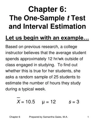
Chapter 6: The One-Sample t Test and Interval Estimation Let us begin with an example… Based on previous research, a college instructor believes that the average student spends approximately 12 hr/wk outside of class engaged in studying. To find out whether this is true for her students, she asks a random sample of 25 students to estimate the number of hours they study during a typical week. X = 10.5 μ = 12 s = 3 Prepared by Samantha Gaies, M.A.
The One-Sample t Test • When σ is known, we can use the normal distribution to obtain our critical values. • When σis not known and Nis very large, we can still use the z score for groups by using s to estimate σ: • However, if σ is not known andN is not very large, we need to use the t distributions to find our critical values: Prepared by Samantha Gaies, M.A.
The t Distributions • First used for significance testing by William Gosset, who published under the pseudonym, Student. • They are bell-shaped, symmetrical distributions with asymptotic tails and a mean of 0. • They are more leptokurtic (sharper peak in the middle with fatter tails) than the normal distribution, but their exact shape depends on the degrees of freedom for the distribution (df). • In the one-group case, df = N – 1. • There are tables for the t distributions that list critical values for common levels of alpha for one- or two-tailed tests. Prepared by Samantha Gaies, M.A.
The One-Sample t Test: Example Completed • Let us calculate t for the example in the first slide. First, • Next, • To find critical t, first note that df = N – 1 = 25 – 1 = 24. • For a .05, two-tailed test, tcrit(24) = 2.064. • The magnitude (i.e., absolute value) of the calculated t is 2.5, which is larger than the critical t, so the null hypothesis can be rejected. The college instructor can conclude that her students study fewer hours than a population that averages 12 hours per week. Prepared by Samantha Gaies, M.A.
The Relation between Sample Size and the One-Sample t Test • As Nincreases (all else constant): • the standard error decreases • the obtained t value increases • the critical t value decreases (until it equals the corresponding value of z) • the chance of attaining statistical significance increases Assumptions of the One-Sample t Test • Conclusions are valid only if the following assumptions are met: • Independent random sampling • Normal distribution (especially when N is small) • Standard deviation of the sample equals that of the comparison population • Conclusions are threatened by the lack of a control group. Prepared by Samantha Gaies, M.A.
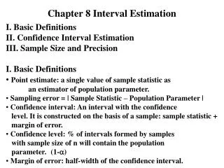
Estimating the Population Mean • Point estimate • A single value is chosen as a best guess of a population parameter. • The mean of a random sample is the best point estimate of the population mean. • Interval estimate • Determines a range of values within which we have a certain amount of confidence that the population parameter falls. • Such an interval is called a confidence interval (CI).The most common amount of confidence associated with a CI is 95%. • The typical CI is symmetrical with the point estimate (e.g., the sample mean) placed at the center. Prepared by Samantha Gaies, M.A.
Confidence Intervals • If you create many, many 95% CIs, about 95% of them will be “hits”; that is, in 95% of the cases, the interval will actually contain the population mean. • The other 5% of the cases will be “misses” (analogous to Type I errors). • The width of a confidence interval is affected by: • Sample size (as sample size increases, all else equal, the width of the CI decreases). • Standard deviation of the sample (larger SDs produce wider CIs). • The amount of confidence (as the percentage of confidence increases, the width of the CI increases). Prepared by Samantha Gaies, M.A.
How to Construct a Confidence Interval for the Population Mean • Select the sample size (usually based on economic considerations). • Select the level of confidence (usually 95% or 99%). • Select the sample randomly, collect the data, and calculate the mean and SD of the sample. • Calculate the limits of the interval; for small samples, this can be done con-veniently by solving the one-sample t test formula for the population mean, as shown below: Prepared by Samantha Gaies, M.A.
More about Confidence Intervals • Uses: • One sample z or t tests are not common, but CIs for the mean have many uses (e.g., opinion polls and election polls). • You get null hypothesis testing as a free by-product (any value for the population mean that is not included in the 95% CI would be rejected as the value for the null hypothesis with a .05, two-tailed test). • Cautions • The assumptions of the one-sample t test apply as well to their corresponding CIs. • CIs based on small samples suffer from large standard errors, because they are divided by a small N. Moreover, the critical t values upon which CIs are based grow larger as the sample size decreases, further widening the CI. Prepared by Samantha Gaies, M.A.
The z Test for a Proportion • To test a proportion, calculate its z score with the following formula: where • P = the proportion observed in a sample • π = the hypothesized value of the population proportion • N = number of cases in the sample • The denominator of the above formula is called the standard error of a proportion, and it is symbolized as σP Prepared by Samantha Gaies, M.A.
The Confidence Interval for a Population Proportion (π) • You can calculate the CI for a propor-tion by means of the formula below: • Unfortunately, we need to know the value of π to find σP, and that is the value that we are trying to estimate. • The solution is to use the P from our sample as an estimate of π in calcula-ting σP, as in the following formula: • The use of P to estimate π is accep- table if the sample size is fairly large. Prepared by Samantha Gaies, M.A.