ESTIMATION AND TEST OF HYPOTHESES: One- sample, two- sample

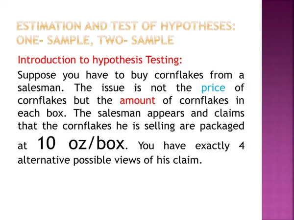
ESTIMATION AND TEST OF HYPOTHESES: One- sample, two- sample Introduction to hypothesis Testing: Suppose you have to buy cornflakes from a salesman. The issue is not the price of cornflakes but the amount of cornflakes in each box. The salesman appears and claims that the cornflakes he is selling are packaged at 10 oz/box. You have exactly 4 alternative possible views of his claim.

Introduction…

Introduction… If you think he is honest you would just go ahead and order your cornflakes from him. You may, however, have one the other views, he is i)CONSERVATIVE or ii)LIAR or iii)CLUELESS. The position you hold regarding the salesman can be any one of these but not more than one. You can’t assume he is liar and conservative ieμ < 10 oz and μ > 10 oz , at the same time.

Introduction… Proper use of scientific method will allow you to test one of these alternative positions through a sampling process. Remember you can choose only one to test. How would you decide ? ?????

Introduction… CASE 1: Testing the salesman is conservative Suppose the salesman is remarkably shy and seems to lack self confidence. You feel from his general conduct that he is being conservative in his claim of 10 oz/box. The situation can be summarized with a pair of hypothesis – actually a pair of predictions. A) The salesman’s claim and the prediction we will directly test. It is usually calledHo or null hypothesis. In this case Ho: μ=10 oz.

Introduction… B) The second is called the alternative or research hypothesis which is your belief or position. The alternative hypothesis in this case is Ha: μ > 10 oz. By writing the null hypothesis as Ho: μ≤ 10 oz. Predictions take the following forms Ho: μ≤ 10 oz (null hypothesis) Ha: μ > 10 oz (alternative hypothesis) And we have generated two mutually exclusive and all-inclusive possibilities. Therefore, either Ho or Ha will be true, but not both.

Introduction.. Hypothses • A. Salesman’s claim(Ho) • B. Customer’s belief or position (Ha)

Introduction… In order to test the salesman’s claim (Ho) against your views (Ha), you decide to do a small experiment. You select 25 boxes of cornflakes from a consignment and carefully empty each box, weigh and record its contents. This experimental sampling is done after you have formulated the two hypotheses. If the first hypothesis were true you would expect the sample mean of the 25 boxes to be close to or less than 10 oz.

Introduction… If the second hypothesis were true you would expect the sample mean to be significantly greater than 10 oz. We have to think about what significantly greater means in this context. In statistics significantly less or more or different means that the result of the experiment would be a rare result if the null hypothesis were true. In other words, the result is far enough from the prediction in the null hypothesis that we feel that we must reject the truthfulness of the hypothesis.

Introduction… The idea leads to the problem of what is a rare result or rare enough result to be sufficiently suspicious of the null hypothesis. For now we will say if the result could occur by chance less than 1 in 20 times if the null hypothesis were true. When we will reject the null hypothesis and consequently accept the alternative ones. Let’s now look at how this decision making criterion works in CASE 1.

Introduction… Ho : μ≤ 10 oz Ha : μ > 10 oz n= 25 and assume and is widely known.

Introduction…. Suppose the mean of your 25 box sample is 10.36 oz. Is that significantly different from (>) 10 oz so that we should reject the claim of 10 oz stated in Ho. Clearly it is greater than 10 oz but is this mean rare enough under the claim of μ≤ 10 oz for us to reject the claim. To answer this question we will use the standard normal transformation to find the probability of ≥10.36 oz when the mean of the sampling distribution of is 10 oz. If this probability is less than 0.05 (1 in 20), we consider the result to be too rare for acceptance of Ho.

Introduction… CASE II: Testing that the salesman is a cheat Suppose our salesman is a fast and smooth talker with fancy cloths and a new sports car. Your view might be that cornflakes salesman only gain this type affluence through unethical practices. You think this guy is cheat. Your null hypothesis is Ho: μ≥ 10 oz and your alternative hypothesis is Ha:μ < 10 oz . Notice that the two hypothesis are again mutually exclusive and all inclusive and that the equal sign is always in the null hypothesis.

Introduction….. It is the null hypothesis (the salesman’s claim) that will be tested. Ho : μ≥ 10 oz Ha : μ < 10 oz. Suppose you again sample 25 boxes to determine the average weight. The question you want to answer and the predictions (Ho, Ha) stemming from that question are again formulated before the sampling is done,

Introduction… n = 25, oz and again we find = 10.36 oz. How does this result fit our predictions ? If Ho is false, we expect the mean to be significantly less than 10 oz.

Introduction… CASE III: Testing that the salesman is clueless The last case is somewhat different from the first in that we really don’t know whether to expect the mean of the sample to be higher or lower than the salesman’s claim. The salesman is new on the job and does not know his product very well. The claim of 10 oz per box is what he has been told, but you don’t have a sense that he is either overly conservative (CASE I) or dishonest (CASE II). Your alternative hypothesis here is less focused.

Introduction… It becomes that the mean is different from 10 oz. The prediction become Ho: μ = 10 oz Ha : μ ≠ 10 oz. Under Ho we expect to be close to 10 oz, while under Ha we expect to be different from 10 oz in either direction ie significantly smaller or significantly larger than 10 oz.

Typical steps in a statistical test of hypothesis • State the problem: should I buy cornflakes from salesman? • Formulate the null and alternative hypothesis Ho : μ = 10 oz Ha : μ ≠ 10 oz 3. Choose the level of significance. This means to choose the probability of rejecting a true null hypothesis. We choose 1 in 20 in our cornflakes example, that is, 5% or 0.05. When Z was so extreme as to occur less than 1 in 20 times if Ho were true, we rejected Ho.

Typical steps… 4. Z is calculated as Determine the appropriate test statistic. Here we mean the index whose sampling distribution is known, so that objective criteria can be used to decide between Ho and Ha. In the cornflakes example we used a Z transformation because under the Central Limit Theorem was assumed to be normally or approximately normally distributed and the value of was known.

Typical steps… 5. Calculate the appropriate test statistic. Only after the first four steps are completed , can one do the sampling and generate the so-called test statistic. Here Z=

Typical steps… 6. Determine the critical values for the sampling distribution and appropriate level of significance. For the two tailed test and level of significance of 1 in 20 we have critical values of + 1.960 (C.3 Tab). These values or more extreme ones only occur 1 in 20 times if Ho is true. The critical values serve as cutoff points in the sampling distribution for regions to reject Ho.

Typical steps…. 7. Compare the test statistic to the critical values. In a two-tailed test, the CV’s = + 1.960 and the test statistic is 1.8, so - 1.960<1.8<1.960. 8. Based on the comparison in step 7, accept or reject Ho. Since Z falls between the critical values, it is not extreme enough to reject Ho. 9. State your conclusion and answer the question posed in step 1. SO WE ACCEPT HO.

Type I vs Type II error in hypothesis testing Because the predictions in Ho and Ha are written so that they are naturally exclusive and all inclusive, we have a situation where one is true and the other is automatically false. When Ho is true, then Ha is false. • If we accept Ho we have done the right thing • If we reject Ho we have made an error This type of mistake is called a Type I error

Type I vs Type II error When Ho is false , then Ha is true • If we accept Ho, we have made an error • If we reject Ho, we have done the right thing The second type of mistake is called Type II error

Example 1. A forest ecologist studying regeneration of rain forest communities in gaps caused by large tree falling during storms, read the stinging (bow) tree, Dendrocnideexcelsa, seedlings will grow 1.5m/yr in direct sun light in each gap. In the gaps in her study plot she identified 9 specimens of this species and measured them in 2009and again 1 yr later. Listed below are the changes in height for the nine specimens.

t-test… Do her data support the published contention that seedlings of this species will average 1.5 m of growth per yr in direct sun light ? 1.9 2.5 1.6 2.0 1.5 2.7 1.9 1.0 2.0 Solution Hypothesis : Ho: μ = 1.5 m/yr Ha: μ ≠ 1.5 m/yr

t-test… If the sample mean for 9 specimens is close to 1.5 m/yr we will accept Ho. If sample mean is significantly larger or smaller than 1.5 m/yr we will accept Ha (reject Ho). To test significant difference, it means that they are so rare that they would occur by chance less than 5% of the time, if Ho is true ieα = 0.05. Test statistic will be

t-test… Here, n=9, s2 =0.260 m2 , s= 0.51 and Clearly t-value of 2.35 is not zero but it is far enough away from zero so that we can comfortably reject Ho. With a predetermined α level of 0.05 we must get a t-value far enough from zero that would occur <5% of the time if Ho is true.

t-test… From Tab C.4 we have the following sampling distribution for t with v=n-1= 8 and α=0.05 for a two tailed test. t=2.35 reject reject 0.025 0.025 accept +2.306 -2.306 0

t-test… If Ho is true and we sample hundreds or thousands of times with samples of 9 species and each time we calculate the t-value for the sample, these t-values would form a distribution with the shape indicated above. 2.5% of the samples would generate t-values below -2.306 and 2.5% of the samples would generate t values above 2.306. So values as extreme as + 2.306 are rare if Ho is true.

t-test… The test statistic in this sample is 2.35 and since 2.35>2.306, the result would be considered rare for a true null hypothesis. We reject Ho based on this comparison and conclude that average growth of stinging trees in direct sun light is different from the published value and is, in fact, greater than 1.5 m/yr. Rejecting Ho may lead to a Type I error.

Example: Two sample test Watching an infomercial on TV you hear the claim that without changing your eating habits, a particular herbal extract when taken daily will allow you to loose 5lb in 5 days. You decide to test this claim by enlisting 12 of your classmates into an experiment. You weigh each subject, ask them to use the herbal extract for 5 days and then weigh them again. From the results recorded below, test the infomercial’s claim of 5 lb lost in 5 days.

Exam. Two sample test

Exam: two sample test Solution: Because the data are paired we are not directly interested in the values presented above, but are interested in the differences or changes on the pairs of members. Think of data as in groups For the paired data here we wish to investigate the differences or di’s where X11-X21 = d1, X12-X22 = d2, X1n-X2n =dn

Exam: Two sample test Expressing the data set in terms of these differences di’s, we have the following table. Note importance of sign of these differences

Exam: two sample test The infomercial claim of a 5 lb loss in 5 days could be written Ho: μB- μA = 5lb but Ho: μd = 5lb is somewhat more appealing Ho: μd = 5 lb Ha: μd ≠ 5 lb Choose α = 0.05, since the two columns of data collapse into one column of interest, we treat these data now as a one sample experiment.

Exam: two sample test There is no preliminary F test and our only assumption is that the di’s are approximately normally distributed. The test statistic for the paired sample t test is With v = n-1, where n is number of pairs of data points.

Exam: two sample test, Here = 3.8 lb, sd = 4.1 lb, n=12. We expect this statistic to be close to 0 if Ho is true ie the herbal extract allows you to loose 5 lb in 5 days. We expect this statistic to be significantly different from 0 if the claim is false.

Exam: two sample test With v= n-1= 12-1 =11. The critical value for this left tailed test from Tab C.4 is t0.05(11)= -1.796. Since -1.796<-1.01 the test statistic does not deviate enough from expectation under a true Ho that you can reject Ho. The data gathered from your classmates support the claim of an average loss of 5 lbs in 5 days with the herbal extract. Because you accept Ho here, you may be making a Type II error (accepting a false Ho), but we have no way of quantifying the probability of this type of error.

Example 3 An expt. was conducted to compare the performance of two varieties of wheat, A and B. Seven farms were randomly chosen for the expt. and the yields in metric tons per hectare for each variety on each farm were as follows;

Example 3… • Why do you think both varieties were on each farm rather than testing variety A on seven farms and variety B on seven different farms? • Carry out a hypothesis test to decide whether the mean yields are the same for the two varieties.

Example 3… Solution: The expt. was designed to test both varieties on each farm because different farms may have significantly different yields due to differences in i) soil characteristics ii) micro climate iii) cultivation practices “Pairing” the data points accounts for most of the “between farm” variability and should make any difference in yield due solely to what variety.

Example 3… The hypotheses are Ho : μA – μB or μd = 0 Ha : μd ≠ 0 Let α = 0.05.Then ton/hectare n =7 and andsd = 0.41 ton/hectare.

Example 3… With v=7-1=6 . The critical values from Tab C.4 are t0.025(6)= -2.447 and t0.975(6) = 2.447. Since -2.447<1.94<2.447 the test statistic does not deviate enough from 0, the expected t value if Ho is true, to reject Ho. From the data given we can not say that the yields of varieties A and B are significantly different.

Chi-square test Example: A geneticist interested in human population has been studying growth patterns in US males since 1900. A monograph written in 1902 states that the mean height of adult US males is 67.0 inch with a standard deviation of 3.5 inch. Wishing to see if these values have changed over the 20th century the geneticists measured a random sample of adult US males and found that = 69.4 inch and s = 4.0 inch. Are these values significantly different from the values published in 1902?

Chi-square… Solution: There are two questions here – one about the mean and the second about the standard deviation or variance. Two questions require two sets of hypotheses and two test statistics. For the question about means, the hypotheses are Ho : μ = 67.0 inch Ha : μ ≠ 67.0 inch

Chi-square… With n = 28 and α = 0.01. This is a two tail test with the question and hypotheses (Ho and Ha) formulated before the data were collected or analyzed. Using an α level of 0.01 for v= n-1= 27, we find the critical values to be ± 2.771 (Tab C.4).

Chi-square… Since 3.16>2.77, we reject Ho and say that modern mean is significantly different from that reported in 1902 and , in fact, is higher than the reported value (because the t-value falls in the right hand tail). P (Type I error)< 0.01. For the question about variance, the hypotheses are Ho: Ha :

Chi-square…. Here n=28. Then The question about variability is answered with a Chi-square statistic. The value is expected to be close to 27 (n-1), if Ho is true and significantly different from 27, if Ha is true.

Chi-square… From Table C.5 using an alpha level of 0.01 for v = 27, we find the critical values for to be 11.8 and 49.6. Since 11.8<35.3<49.6 we do not reject Ho here. There is not statistical support for Ha. The p value here for p is between 0.500(31.5) and 0.250(36.7) indicating the calculated value is not a rare event under the null hypothesis.

ESTIMATION AND TEST OF HYPOTHESES: One- sample, two- sample