Download
1 / 16
250 likes | 628 Vues
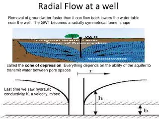
Radial Flow at a well. Removal of groundwater faster than it can flow back lowers the water table near the well. The GWT becomes a radially symmetrical funnel shape. called the cone of depression . Everything depends on the ability of the aquifer to transmit water between pore spaces.

E N D
Radial Flow at a well Removal of groundwater faster than it can flow back lowers the water table near the well. The GWT becomes a radially symmetrical funnel shape called the cone of depression. Everything depends on the ability of the aquifer to transmit water between pore spaces Last time we saw hydraulic conductivity K, a velocity, m/sec
Transmissivity and Permeability • Transmissivity is a term applied to confined aquifers. It is the product of the hydraulic conductivity K and the saturated thickness b of the aquifer. T = K [m/day] . b [m] • Permeability symbol k, “little k” has units [m2] k = Km/rg where m is the dynamic viscosity [kg/m.sec] and K has units m/sec
Water Production Well Casing, screen, centrifugal pump Outer casing >12” above grade with cement grout, lower casing with grout seal, pump in screen, sand gravel pack, developed
Radial Flow • The drawdown of the GWT during flow from a well varies with distance, the cone of depression. If we want to know the difference in height h of the GWT at different distances r away from the well, we can sum thin cylinders of water around the well. Cylinders have lateral area 2pr . height. Grundfos submersible pump
Radial Flow- Confined Aquifer [m.m.(m/sec).m/m] • If the aquifer is confined, the cylinder has height h = b, and Darcy’s Equation for flow can be integrated for a solution for r and h: Area xK x dh/dr To solve we integrate (get the total area), i.e. we add up many thin cylinders Separate the variables r and h sum terms in r = constants x sum terms in h d ln r = 1/r dr d h = dh so: Solve the above for Q
Radial Flow- Confined AquiferSolve for T • If we solve for T=Kb we get: We will go through Example 8-4.
Radial Flow- Unconfined Aquifer • If the aquifer is unconfined, the cylinder has height h, and Darcy’s Equation for flow can be integrated for a solution for r and h as well. The extra h gives a little different solution: Such expressions can be solved for K
Radial Flow- Unconfined AquiferSolve for K • If we solve for K we get: We will go through Example 8-5.
Slug Tests • These use a single well for the determination of aquifer formation constants • Rather than pumping the well for a period of time, a volume of pure water is added to the well and observations of drawdown are noted through time • Slug tests are often preferred at hazardous waste sites, since no contaminated water has to be pumped out and disposed of.
Bouwer and Rice Slug Test begins middle of page 540 4th edition rc= radius of casing y0 = vertical difference between water level inside well and water level outside at t = 0 yt = vertical difference between water level inside well and water table outside (drawdown) at time t Re = effective radial distance over which y is dissipated; varies with well geometry rw = radial distance to undisturbed portion of aquifer from centerline (includes thickness of gravel pack) Le = length of screened, perforated, or otherwise open section of well, and t = time
A screened, cased well penetrates a confined aquifer. The casing radius is rc = 5 cm and the screen is Le = 1 m long. A gravel pack 2.5 cm thick surrounds the well so rw = 7.5 cm. A slug of water is injected that raises the water level by y0 = 0.28 m. The change in water level yt with time is as listed in the above table. TODO: Given that Re is 10 cm, calculate K for the aquifer. t (sec)yt(m) 1 0.24 2 0.19 3 0.16 4 0.13 6 0.07 9 0.03 13 0.013 19 0.005 20 0.002 40 0.001 Example from Figure 8-23b
First we estimate the 1/t ln(y0/yt) Data for y vs. t are plotted on semi-log paper as shown. The straight line from y0= 0.28 m to yt = 0.001 m covers 2.4 log cycles. The time increment between the two points is 24 seconds. To convert the log10 cycles to natural log (ln) cycles, a conversion factor of 2.3 is used. Thus, 1/t ln(y0/yt) = 2.3 x 2.4/24 = 0.23. 0.3 0.2 4/10ths of a log cycle, read as a proportion of the length of one log cycle, NOT on the log scale second log cycle first log cycle
Log10 to ln • Consider the number 10. • Log10 (10) = 1 because 101 = 10 • ln (10) = 2.3 • ln (10) / Log10 (10) = 2.3/1
Reading log marks if not labeledAlso, the meaning of “one cycle”“half a cycle” etc. One cycle Half a cycle
The Solution Using this value (0.23) for 1/t ln(y0/yt) in the Bouwer and Rice equation gives: K = [(5 cm)2 ln(10 cm/7.5 cm)/(2 x 100 cm)](0.23 sec-1) and, K = 8.27 x 10⁻³ cm/s rc = 5 cm Le = 1 m Gravel pack = 2.5 cm thick So R = rw = 2.5 + 5 = 7.5cm y0 = 0.28 m. Re is 10 cm 1/t ln(y0/yt) = 0.23 from the previous slides.
More Examples • As usual we will do examples and similar homework problems.