Download
1 / 30
300 likes | 465 Vues
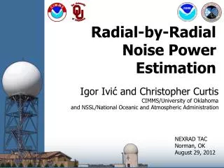
the University of Oklahoma. Radial-by-Radial Noise Power Estimation. Igor Ivić and Christopher Curtis CIMMS/University of Oklahoma and NSSL/National Oceanic and Atmospheric Administration. NEXRAD TAC Norman, OK August 29, 2012. Motivation.

E N D
the University of Oklahoma Radial-by-RadialNoise Power Estimation Igor Ivić and Christopher Curtis CIMMS/University of Oklahoma and NSSL/National Oceanic and Atmospheric Administration NEXRAD TAC Norman, OK August 29, 2012
Motivation • Incorrect noise power measurements can lead to: • Reduction of coverage when noise power is overestimated • Case in most radar sites • Radar product images cluttered by noise speckles if the noise power is underestimated • Usually occurs in cases of strong interference • Biased meteorological variables at low to moderate SNR + the system gain can change within minutes … • Blue-sky noise used to produce system noise power • Adjusted for lower elevations using correction factors • For each elevation, the same value is used at all azimuths • However, noise drifts with time and varies with antenna position in azimuth and elevation
Solution • Radial-by-radial noise power estimation technique provides the solution • Estimate receiver noise power at each antenna position • Noise power needs to be computed in real-time (i.e., from data containing mixed signals and noise) • BUT HOW DO YOU DO THAT?
Radial-by-Radial Noise Estimation • History • First Version presented at ERAD in September 2010 • required rough initial noise value • Second version presented at AMS in January 2011 • no rough initial noise value required • Algorithm description of the latest version delivered to the ROC in May 2012 • includes high gradient signal removal • simplified so it operates only on the measured powers • The technique has been in use on the NWRT since June 2011
Technique Description Expert noise power Ne determined visually Used to assess the technique accuracy
Power Profile of Test Data Received power as a function of range at the elevation angle of 0.5 deg. The expert noise power (Ne) is indicated with a grey line.
Step 1:Strong Point Clutter Rejection BEFORE POINT CLUTTER REJECTION AFTER POINT CLUTTER REJECTION Gate at location k is considered to contain point clutter if its power is much larger than the power at surrounding gates
Step 2: Detect Flat Sections Notice that the local range variance is smaller in noise regions • The flat sections of the power profile are identified as this is an indication of the potential signal-free regions • This is done by estimating local variance along range • (local range variance at k < threshold) => range gate at k considered potentially signal-free
Step 2: Flat Sections Detected The mean power is computed for each group of contiguous range gates classified as signal-free Out of those, the smallest one is taken to be the intermediate noise power estimate (Nint)
Step 3: SNR Censoring Using Nint Discard all samples at range locations for which the power estimate is larger than the threshold (THR(M)xNint)
Step 3: Output after Nint SNR Censoring Mean power/expert noise = -0.216 dB Mean power/expert noise = 0.243 dB Potential signal regions SNR profile of data after discarding samples at range gates where power estimate is larger than the threshold.
Step 4: Apply "range persistence" Filter • Detects larger sample powers that exhibit continuity in range • Finds 10 or more consecutive power values larger than the median power
Steps 5&6: Update Active Range Gates and Censor using SNR Threshold • Discard the samples marked by the range persistence filter • Compute the mean power of the remaining samples • Perform SNR censoring Mean power/expert noise = 0.1586 dB Mean power/expert noise = -0.2376 dB
Step 7: Apply Running Sum Filter After 1 iteration mean power/expert noise = -0.3 dB After 1 iteration mean power/expert noise = -0.0043 dB • A running sum is performed over the array of remaining powers • makes regions with weak signals visible
Accuracy Assessment • To assess the accuracy • estimated noise is subtracted from all powers • simulated noise is artificially added to the real data Algorithm failed to produce noise estimate 43 times out of 155164 (0.03%) BIAS = -4×10⁻³ dB or -0.086% of the true noise STD = 5.3×10⁻² dB or 1.22% around the mean
SUMMARY Radial-by-radial noise power estimation technique accurately produces noise power measurements in real-time! GREAT SUCCESS!
Benefits of Radial-by-Radial Noise Estimation • Comparison between the measured noise power and legacy noise power • Can see effects from man-made (KVNX) and mountain (KPDT) clutter • Will use data from these cases to illustrate benefits KVNX: Vance AFB, OK KPDT: Portland, OR 0.9 dB 4 dB 1 dB 1 dB
Reflectivity Coverage KPDT Data with Legacy Noise (0.9°, VCP 12, Cut 3)
Reflectivity Coverage KPDT Data with Measured Noise (0.9°, VCP 12, Cut 3) Coverage increased by 18%
69.6% of vestimates with legacy noise are valid (i.e., v > 0) 89.0% of vestimates with measured noise are valid Invalid Spectrum Width Values KPDT Data with Legacy vs. Measured Noise (0.9°, VCP 12, Cuts 1&2) 49.4% IMPROVEMENT IN THE NUMBER OF VALID ESTIMATES
Invalid Correlation Coefficient Values KVNX Data with Legacy vs. Measured Noise (0.5°, VCP 11, Cut 1) • 78% of |hv(0)| estimates with legacy noise are less than one • 84.48% of hv(0) estimates with measured noise are less than one 14.9% IMPROVEMENT IN THE NUMBER OF VALID ESTIMATES
Effects on ZDR • Differential reflectivity is estimated as where Nh and Nv are errors in noise floors • Using perturbation analysis, we get • If errors in H and V are of different sign they add up, otherwise they may cancel
Contribution of Noise Error to ZDR Bias KVNX Nh = -80.7 dBm & Nv = -81.2 dBm Nh = -0.9 dB & Nv = -1 dB KPDT Nh = -80.6 dBm & Nv = -80.3 dBm Nh = -4 dB & Nv = -1 dB • In the current system, noise errors are significant contributors to the ZDR bias for low to moderate SNR • Real-time noise estimates eliminate this contribution because of accurate measurements (i.e., Nh 0, Nv 0)
Summary • Improved data quality with measured noise: • Increased coverage for all moments and dual-polarization variables • Reflectivity – decreased bias • Spectrum Width (v) – decreased bias and increased number of valid estimates • Correlation coefficient (|hv(0)|) – decreased bias and increased number of valid estimates • Differential reflectivity (ZDR) – decreased bias • Accurate noise measurement is crucial for keeping measurement biases within acceptable levels
Conclusions • Accurate noise estimation accounts for noise variations due to: • Changes in system gain (Melnikov et al.) • Radiation caused by clutter, storms and man made objects • These noise variations can lead to: • Reduction of coverage when noise power is overestimated • Radar product images cluttered by noise speckles if the noise power is underestimated • Biased meteorological variables at low to moderate SNR (e.g., differential reflectivity and correlation coefficient) • The current system calibration does NOT address these issues! • Radial-by-Radial Noise Estimation eliminates or greatly mitigates all of these issues stemming from incorrect noise power measurements.
Reflectivity Coverage KVNX Data with Legacy Noise (0.5°, VCP 11, Cut 1)
Reflectivity Coverage KVNX Data with Measured Noise (0.5°, VCP 11, Cut 1) Coverage increased by 6.18%
Invalid Spectrum Width Values KPDT Data with Legacy Noise (0.5°, VCP 12, Cuts 1&2)
Invalid Spectrum Width Values KPDT Data with Measured Noise (0.9°, VCP 12, Cuts 1&2)