Automatic Ice Thickness Estimation from Polar Subsurface Radar Imagery
350 likes | 633 Vues
Automatic Ice Thickness Estimation from Polar Subsurface Radar Imagery. Gladys Finyom Michael Jefferson Jr. MyAsia Reid Christopher M. Gifford Eric L. Akers Arvin Agah. Overview. Introduction Background/ Related Works Overview of Remote Sensing Challenges of Processing Radar Imagery

Automatic Ice Thickness Estimation from Polar Subsurface Radar Imagery
E N D
Presentation Transcript
Automatic Ice Thickness Estimation from Polar Subsurface Radar Imagery • Gladys Finyom • Michael Jefferson Jr. • MyAsia Reid • Christopher M. Gifford • Eric L. Akers • Arvin Agah
Overview • Introduction • Background/ Related Works • Overview of Remote Sensing • Challenges of Processing Radar Imagery • Ice Thickness Estimation from Radar Data • Methods • Edge Detection and Following Approach • Active Contour; Cost Minimization Approach • Experimental Results • Conclusion
Introduction • Remote sensing methods: • CReSIS uses Radar and Seismic/acoustic to acquire subsurface data from a remote location. (i.e., surface, air, or space). Radar and Acoustic sensors: • used to gather data about the internal and bottom layers of ice sheets, from the surface. Other Examples: • Satellite-based imagery, and identification of events.
Introduction • Surfaced-based and Airborne radio echo sounding of Greenland and Antarctica ice sheets: • Determine ice sheets thickness • Bedrock Topography (smooth, rough) • Mass Balance of large bodies of ice. Challenges in Radar Sounding: • Rough surface interface • Stages of melting (top, inside) • Variations of ice thickness, topography Processing Data: • Requires knowledge about sensing medium • Ultimately used for scientific community Greenland's ice sheet NASA/Rob Simmon
Introduction • Goal: • Focus on automating task of estimating ice thickness. Process: • Identifying and accurately selecting of ice sheet’s surface, interface between the ice, and the bedrock. Knowing the surface and bedrock in the radar images: • helps compute the ice thickness. • help studies relating to the ice sheets, their volume, and how they contribute to climate change. Four outlet Glaciers studied by CReSIS researchers. Leigh Stearns
Overview of Radar Remote Sensing • Radars transmit energy in form of a pulse from an antenna, energy reflects off of target(s), and is received by an antenna. • Distance measured based on energy travel time back and forth from the targets. • Gives reflection intensity and depth information about the targets. • Ground Penetrating Radar (GPR) able to observe properties of subsurface, ranging from soil, rock, sand and ice. • When data is collected, the targets are internal layering in the ice sheets which have a strong echo return from the bedrock beneath the ice. • Interface (3.5 km or >) below the surface. • Requires great transmit power and sensitive receive equipment because of energy loss within ice and with depth.
Column Pixel Overview of Radar Remote Sensing • Each measurement is called a radar trace, and consist of signals, representing energy due to time. The larger time correlates with deeper reflections. • In an image, a trace is an entire column of pixels, each pixel represents a depth. • Each row corresponds to a depth and time for a measurement, as the depth increases further down.
Overview of Radar Remote Sensing • A flight segment consist of a collection of traces which represent all the columns of the image, from the beginning (left) to the end (right) during flight. • A pixel width represents the track distance between traces, and depend on the speed of the aircraft during the survey. • The flight segment is called an Echogram.
Overview of Radar Remote Sensing • The Energy from the radar into the ice changes in dielectric properties (air to ice, ice to bed rock) and causes the energy to reflect back. • Water surrounded by the ice, and frozen ice against the bedrock both represent a strong reflecting interface. • To determine whether each is present, it depends on the radar and its setting. Reflection intensities are strongest at the surface and weaker because of depth. Depth increases from left to right.
Example Radar Echogram: Greenland 05/28/2006 Figure shows radar echogram over an ice sheet, illustrating the reflection of internal layers and the bedrock interface beneath the ice sheet.
Challenges of Processing Radar Imagery • Automated processing and extraction of high level information from radar imagery is challenging. • Noise is usually electromagnetic interference from other onboard electronics. • Low magnitude, faint, or non-existent bedrock reflections occur: • Specific radar settings • Rough surface/bed topography • Presence of water on top/internal to the ice sheet. • This produces gaps in the bedrock reflection layer which must be connected to construct an adjacent layer for the completion of ice thickness estimation.
Challenges of Processing Radar Imagery • Backscatter introduce clutter and contributes to regions of images incomprehensible. • In addition, bed topography varies from trace to trace due to rough bedrock interfaces from extended flight segments. • Lastly, a strong surface reflection can be repeated in an image, surface multiple due to energy reflecting off of the ice sheet surface and back again. • If there is a time difference between the first and second surface return, the surface layer will repeat in an image, at a lower magnitude with an identical shape.
Ice Thickness Estimation from Radar • Along with raw data values, and GPS location measurements, ice thickness is needed for scientist to: • study mass balance • sea level rise • Environmental/ human impacts • Ice thickness is computed by selecting the surface and bedrocks reflections in pixel/depth coordinates, for each trace, and subtracting their corresponding depths. • Several experts had select the layers using custom software.
Ice Thickness Estimation from Radar • The surface is selected based on the first and largest reflection return. • The bedrock, is more challenging due to buried noises. • Experts tend to skip traces to speed up the process. • This causes errors, and require more time to estimate ice thickness in a single file. • Thousands of images need work, and the manual approach is not sufficient. Figure shows CReSIS picking software, the surface return is fully picked, while bedrock return is partially picked.
Related Work • Internal Layer: • predicts depth in certain layers. • depth and thickness of Eemain Layer in Greenland ice sheet utilized Monte Carlo Inversion flow model to estimate unknown parameters guarded by internal layers. 1,2 Identification: • Layers, contours, and curves are done using image processing, and computer methods. • Adaptive contour snake fitting, where an image is a cost grid, and represents a certain amount of energy. 3,4 • Such approaches have been used in medical imagery (such as MRIs and CAT scans). 5 [3] T. F. Chan, L. A. Vese, Active Contours Without Edges, IEEE Transactions on Image Processing 10 (2) (2001) 266–277. [4] M. Kass, A. Witkin, D. Terzopoulos, Snakes: Active Contour Models, International Journal of Computer Vision (1988) 321–331. [5] J. Kratky, J. Kybic, Three-Dimensional Segmentation of Bones from CT and MRI using Fast Level Sets, in: Medical Imaging: Proceedings of the SPIE, Vol. 6914, 2008, pp. 691447–691447–10. [1] S. L. Buchardt, D. Dahl-Jensen, Predicting the Depth and Thickness of the Eemian Layer at NEEM Using a Flow Model and Internal Layers, in: Geofysikdag, 2007. [2] S. L. Buchardt, D. Dahl-Jensen, Estimating the Basal Melt Rate at NorthGRIP using a Monte Carlo Technique, Annals of Glaciology 45 (1) (2007) 137–142.
Edge Detection and Following Approach Introduction • Edge Detection, Thresholding, Edge Following • Surface should be max value in each trace • Bedrock should be the deepest contiguous layer in image Similar Work • Skyline Detector • Growing seeds in the sky • Identify week clouds in sky imagery Our Approach • Trace processed from bottom-up fashion until a strong edge is encountered
Automatic Surface and Bottom Layer Selection Surface Selection • Extracting the location of the ice sheet surface • The depth corresponding to the max value of each trace is selected as location of surface reflection Bottom Selection Preprocessed by: • Detrending • Low-pass filtering • Contrast adjustment Figure: Echogram that has been preprocessed using detrending, low-pass filter, and contrast enhancement Figure: Normalized echogram gradient magnitude, showing the image edges
2D Derivative of Gaussian Kernel Figure: 2D derivative of Gaussian convolution kernels (1.5 ) for computing vertical (left) and horizontal (right) image gradients.
Cleaned Edge Image & Result Image Figure: Cleaned edge image following thresholding, morphological closing and thinning operations Figure: Echogram with overlaid automatically selected surface (top, red) and bedrock (middle, blue) layers using the edge-based method.
Active Contour & Cost Minimization Approach • Similar work - Mars Exploration Rovers (MER)’s automatic sky segmentation system - Further analysis of segmentation • Our Approach Contour technique to fit a contour to the bottom layer
Automatic Surface and Bottom Layer Selection • Surface Selection Same as Edge Detection technique • Bottom Selection - Data preprocessing - EdgeCosts = 1/√(1+Gradient Magnitude) - Creating an Image Gradient for upward force - Adding the edge cost image and upward force image Figure: Edge cost image, enforcing low cost for strong edges and high cost for noise regions
Initialization • The contour is allowed to adapt until it reaches equilibrium • 2N+1 window (N = 50 pixels) is maintained • Window utilized for computing local stiffness to instill continuity and smoothness during adjustment • Determination of Lowest cost (0) pixels and Highest cost pixels (1) • This technique allows the contour to fit to the image and bridge gaps in the bedrock layer Bottom Layer Selection Continues… Figure: Combined edge cost and upward cost images
Contour Cost Window & Active Contour Figure: contour stiffness cost window during processing (left) for the contour’s configuration during the 75th iteration (right), illustrating how the contour is encouraged to make smooth transitions from trace-to-trace.
Final Adjustments • TotalCostWindow(t) = EdgeCosts(s) + α x UpwardCosts(t) + β x ContourStiffnessCosts(t) • The minimal pixel location at each trace is selected as the contour’s starting configuration • If the configuration does not change between iterations, or 500 iterations have been processed, the contour is determined to have reached equilibrium • Ice thickness is computed for each trace by converting pixels for the bedrock selection to a depth in meters and subtracting it from the surface depth for each trace Figure: Echogram with overlaid automatically selected surface(top, red) and bedrock (middle, blue) layers using the active contour method. Green is the initial contour configuration.
Active Contour Configuration Figure: Example contour adaptation sequence throughout processing, illustrating how the contour adapts to the bedrock interface and fits itself to the most salient edge near the bottom of the image
Experimental Results • Processed in Matlab • Data were 15 random subsets of 75 extended flights from Greenland. • Range from 800-3000 rows and 1750-14500 columns (traces). • Previous manual selection method took roughly 45 minutes per file with approx 7500 columns per file. • Automated edge-based method takes 15 seconds per file. • Active contour (snake) method takes 2.5 minutes per file.
Results • We assumed that the human approach was 100% accurate • Selection is considered correct if it is within 5% of the human selection • There are drawbacks with the manual approach
Edge-Based Method • This method differs slightly from the active contour results even though both used same technique • No Continuity Active Contour Method • Method is able to outperform the edge-based method • Takes a little longer to process images • Smooth • Continuous
Edge Method vs. Contour Method Gap in bedrock Contour method bridges the gap
Continued Example Plotted points above the bedrock Active Contour method rids the echogram on non-continuous plotted pixels Plotted pixels below actual bedrock
Continued Example Edge-detection method works better Artifact/Noise in the bedrock layer