Download
1 / 13
140 likes | 248 Vues
Analyze average case performance of programs using the Incompressibility Method with incompressible inputs. Covers formal language theory, combinatorics, fast adder, sorting algorithms like Shellsort, Heapsort, and important results in computer science. Provides insights on average case analysis, lower bounds, and theorem proofs.

E N D
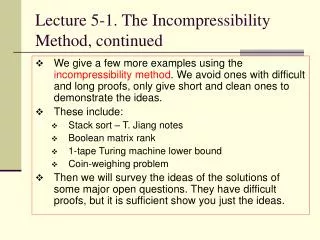
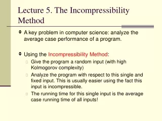
Lecture 5. The Incompressibility Method • A key problem in computer science: analyze the average case performance of a program. • Using the Incompressibility Method: • Give the program a random input (with high Kolmogorov complexity) • Analyze the program with respect to this single and fixed input. This is usually easier using the fact this input is incompressible. • The running time for this single input is the average case running time of all inputs!
Formal language theory • Example: Show L={0k1k | k>0} not regular. By contradiction, assume that DFA M accepts L. Choose k so that C(k) >> 2|M|. Simulate M: 000 … 0 111 … 1 C(k) < |M| + q + O(1) < 2|M|. Contradiction. • Remark. Generalize to iff condition: more powerful & easier to use than “pumping lemmas”. k k stop here M q
Combinatorics • ExampleThere is a tournament (complete directed graph) T of n players that contains no large transitive subtournaments(>1 + 2 log n). Proof by Picture: Choose a random T. • One bit codes an edge. C(T) ³ n(n-1)/2. • If there is a large transitive subtournament, then a large number of edges are given for free! C(T)< n(n - 1)/2 - subgraph-edges + overhead Linearly ordered subgraph. Easy to describe T
Fast adder • Example. Fast addition on average. • Ripple-carry adder: n steps adding n-bit numbers. • Carry-lookahead adder: 2 log n steps. • Burks-Goldstine-von Neumann (1946): logn expected steps. S= xy; C= carry sequence; while (C≠0) { S= SC; C= new carry sequence; } Average case analysis: Fix x, take random y s.t. C(y|x)≥|y| x = … u1 … (Max such u is carry length) y = … û1 …, û is complement of u If |u| > log n, then C(y|x)<|y|. Average over all y, get logn. QED
Sorting • Given n elements (in an array). Sort them into ascending order. • This is the most studied fundamental problem in computer science. • Shellsort (1959): P passes. In each pass, move the elements “in some stepwise fashion” (Bubblesort) • Open for over 40 years: a nontrivial general average case complexity lower bound of Shellsort?
Shellsort Algorithm • Using p increments h1, … , hp, with hp=1 • At k-th pass, the array is divided in hk separate sublists of length n/hk (taking every hk-th element). • Each sublist is sorted by insertion/bubble sort. ------------- • Application: Sorting networks --- nlog2 n comparators.
Shellsort history • Invented by D.L. Shell [1959], using pk= n/2k for step k. It is a Θ(n2) time algorithm • Papernow&Stasevitch [1965]: O(n3/2) time. • Pratt [1972]: O(nlog2n) time. • Incerpi-Sedgewick, Chazelle, Plaxton, Poonen, Suel (1980’s) – worst case, roughly,Θ(nlog2n / (log logn)2). • Average case: • Knuth [1970’s]: Θ(n5/3) for p=2 • Yao [1980]: p=3 • Janson-Knuth [1997]: Ω(n23/15) for p=3. • Jiang-Li-Vitanyi [J.ACM, 2000]: Ω(pn1+1/p) for any p.
Shellsort Average Case Lower bound Theorem. p-pass Shellsort average case T(n) ≥ pn1+1/p Proof. Fix a random permutation Π with Kolmogorov complexity nlogn. I.e. C(Π)≥nlogn. Use Πas input. For pass i, let mi,k be the number of steps the kth element moves. Then T(n) = Σi,k mi,k From these mi,k's, one can reconstruct the input Π, hence Σ log mi,k≥ C(Π) ≥ n logn Maximizing the left, all mi,k must be the same. Call it m. Σ log m = pn log m ≥ Σ log mi,k ≥ nlogn mp ≥ n. So T(n) = pnm > pn1+1/p. ■ Corollary: p=1: Bubblesort Ω(n2)average case lower bound. p=2: n1.5lower bound. p=3, n4/3 lower bound
Heapsort • 1964, JWJ Williams [CACM 7(1964), 347-348] first published Heapsort algorithm • Immediately it was improved by RW Floyd. • Worst case O(nlogn). • Open for 40 years: Which is better in average case: Williams or Floyd? • R. Schaffer & Sedgewick (1996). Ian Munro provided the solution here.
Heapsort average analysis (I. Munro) • Average-case analysis of Heapsort. Heapsort: (1) Make Heap. O(n) time. (2) Deletemin, restore heap, repeat. Williams Floyd log n d d 2 log n - 2d log n + d comparisons/round Fix random heap H, C(H) > n log n. Simulate Step (2). Each round, encode the red path in log n -d bits. The n paths describe the heap! Hence, total n paths, length ³ n log n, d must be a constant. Floyd takes n log n comparisons, and Williams takes 2n log n.
A selected list of results proved by the incompressibility method • Ω(n2) for simulating 2 tapes by 1 (20 years) • k heads > k-1 heads for PDAs (15 years) • k one-ways heads can’t do string matching (13 yrs) • 2 heads are better than 2 tapes (10 years) • Average case analysis for heapsort (30 years) • k tapes are better than k-1 tapes. (20 years) • Many theorems in combinatorics, formal language/automata, parallel computing, VLSI • Simplify old proofs (Hastad Lemma). • Shellsort average case lower bound (40 years)
More on formal language theory Lemma (Li-Vitanyi) Let L V*, and Lx={y: xy L}. Then L is regular implies there is c for all x,y,n, let y be the n-th element in Lx, we have C(y) ≤ C(n)+c. Proof. Like example. QED. Example 2. {1p : p is prime} is not regular. Proof. Let pi, i=1,2 …, be the list of primes. Then pk+1 is the first element in LPk, hence by Lemma, C(pk+1)≤O(1). Impossible. QED
Characterizing regular sets • For any enumeration of *={y1,y2, …}, define characteristic sequence of Lx={yi : xyi L} by Xi = 1 iff xyi L Theorem. L is regular iff there is a c for all x,n, C(Xn|n) < c