BASIC STATISTICAL TOOLS
BASIC STATISTICAL TOOLS. What is Statistics. Statistics refers to the collection , presentation , analysis , and utilization of numerical data to make inferences and reach decisions in the face of uncertainty in economics, business, and other social and physical sciences .

BASIC STATISTICAL TOOLS
E N D
Presentation Transcript
What is Statistics • Statistics refers to the • collection, • presentation, • analysis, • and utilization of numerical data to makeinferences and reach decisions in the face of uncertainty in economics, business, and other social and physical sciences. Statistics is subdivided into descriptive and inferential.
Descriptive statistics Descriptive statistics : Methods of organizing, summarizing, and presenting data in an informative way. EXAMPLE : According to Consumer Reports, Whirlpool washing machine owners reported 9 problems per 100 machines during 1995. The statistic 9 describes the number of problems out of every 100 machines.
Inferential statistics Inferential statistics is the process of reaching generalizationsabout the whole (called the population) by examining a portion (called the sample). A populationis a collection of all possible individuals, objects, or measurements of interest. A sample is a portion, or part, of the population of interest.
EXAMPLE Suppose that we have data on the incomes of 1000 U.S. families. This body of data can besummarized by finding the average family income and the spread of these family incomes above and below theaverage. The data also can be described by constructing a table, chart, or graph of the number or proportion offamilies in each income class. This is descriptive statistics. If these 1000 families are representative of all U.S.families, we can then estimate and test hypotheses about the average family income in the United States as a whole.This is statistical inference.
TYPES OF DATA There are three types of data that are generally available for empirical analysis. 1. Time series 2. Cross-sectional 3. Pooled (A combination of time series and cross-sectional)
TIME SERIES DATA Collected over a period of time, such as the data on: GDP, employment, unemployment, money supply, government deficit. Such data may be collected at regular intervals: Daily (e.g. Stock prices) Weekly (e.g. Money supply) Monthly (e.g. Unemployment rate) Quarterly (e.g. GDP) Annually (e.g. Government budget) This is called the frequency of the data.
TIME SERIES DATA These data may be quantitative in nature (e.g. Prices, income, money supply) Or qualitative in nature (e.g. Male or female, employed or unemployed, married or unmarried, white or black) Qualitative variables are also called dummy or categorical variables.
CROSS-SECTIONAL DATA These are data on one or more variables collected at one point in time For example GDP of European Union Countries in 2010. Government budget deficit of BRIC countries.
POOLED DATA In Pooled data we have elements of both time series and cross-sectional data. For example Unemployment rate for 10 countries for a period of 20 years. (Pooled data) Data on the unemployment rate for each country for the 20 year period (Time series) Data on the unemployment rate for the 10 countries for any single year (Cross-sectional)
2-2 Frequency Distribution • Frequency distribution: A grouping of data into categories showing the number of observations in each category. • The number of classes is usually between 5 and 15.
2-4 Frequency Distribution • Class mark (midpoint): A point that divides a class into two equal parts. This is the average between the upper and lower class limits. • Class interval: For a frequency distribution having classes of the same size, the class interval is obtained by subtracting the lower limit of a class from the lower limit of the next class.
2-4 Frequency Distribution • Class mark (midpoint): A point that divides a class into two equal parts. This is the average between the upper and lower class limits. • Class interval: For a frequency distribution having classes of the same size, the class interval is obtained by subtracting the lower limit of a class from the lower limit of the next class.
2-5 EXAMPLE 1 • Dr. Tillman is the dean of the school of business and wishes to determine the amount of studying business school students do. He selects a random sample of 30 students and determines the number of hours each student studies per week: • 15.0, 23.7, 19.7, 15.4, 18.3, 23.0, 14.2, 20.8, 13.5, 20.7, 17.4, 18.6, 12.9, 20.3, 13.7, 21.4, 18.3, 29.8, 17.1, 18.9, 10.3, 26.1, 15.7, 14.0, 17.8, 33.8, 23.2, 12.9, 27.1, 16.6. • Organize the data into a frequency distribution.
2-6 EXAMPLE 1 continued Consider the classes 8-12 and 13-17. The class marks are 10 and 15. The class interval is 5 (13-8).
2-7 Suggestions on Constructing a Frequency Distribution • The class intervals used in the frequency distribution should be equal. • Determine a suggested class interval by using the formula: i = (highest value-lowest value)/number of classes.
2-8 Suggestions on Constructing a Frequency Distribution • Use the computed suggested class interval to construct the frequency distribution. Note: this is a suggested class interval; if the computed class interval is 97, it may be better to use 100. • Count the number of values in each class.
2-9 Relative Frequency Distribution • The relative frequency of a class is obtained by dividing the class frequency by the total frequency. • The sum of the relative frequencies equals 1. Hours
EXAMPLE 2 The cans in a sample of 20 cans of fruit contain net weights of fruit ranging from 19.3 to 20.9 oz, asgiven in the Table. If we want to group these data into 6 classes, we get class intervals of 0.3 oz [21,0 – 19,2/6 ]= 0,3oz. The weights given in the Table can be arranged into the frequency distributions givenin the next Table.
2-10 Stem-and-Leaf Displays • Stem-and-Leaf Display: A statistical technique for displaying a set of data. Each numerical value is divided into two parts: the leading digits become the stem and the trailing digits the leaf. • Note:An advantage of the stem-and-leaf display over a frequency distribution is we do not lose the identity of each observation.
2-11 EXAMPLE 3 • Colin achieved the following scores on his twelve accounting quizzes this semester: 86, 79, 92, 84, 69, 88, 91, 83, 96, 78, 82, 85. Construct a stem-and-leaf chart for the data.
2-12 Graphic Representation of a Frequency Distribution • The three commonly used graphic forms are • histograms, • frequency polygons, and • cumulative frequency distribution. • Histogram: A graph in which the classes are marked on the horizontal axis and the class frequencies on the vertical axis. The class frequencies are represented by the heights of the bars and the bars are drawn adjacent to each other.
2-14 Histogram for Hours Spent Studying
Frequency Polygon A frequency polygon consists of line segments connecting the points formed by the class midpoint and the class frequency.
2-15 Frequency Polygon for Hours Spent Studying
Cumulative Frequency Distribution A cumulative frequency distribution is used to determine how many or what proportion of the data values are below or above a certain value.
2-16 Cumulative Frequency Distribution For Hours Studying
2-17 Bar Chart • A bar chart can be used to depict any of the levels of measurement (nominal, ordinal, interval, or ratio). • EXAMPLE 3: Construct a bar chart for the number of unemployed people per 100,000 population for selected cities.
2-18 EXAMPLE continued
2-19 Bar Chart for the Unemployment Data
2-20 Pie Chart • A pie chart is especially useful in displaying a relative frequency distribution. A circle is divided proportionally to the relative frequency and portions of the circle are allocated for the different groups. • EXAMPLE 4: A sample of 200 runners were asked to indicate their favorite type of running shoe.
2-21 EXAMPLE continued • Draw a pie chart based on the following information.
2-22 Pie Chart for Running Shoes
MEASURES OF CENTRAL TENDENCY Central tendency refers to the location of a distribution. The most important measures of central tendency are (1) the mean, (2) the median, and (3) the mode.
The Median The median for ungrouped data is the value of the middle item when all the items are arranged ineither ascending or descending order in terms of values: where N refers to the number of items in the population (n for a sample).
The Mode The mode is the value that occurs most frequently in the data set. The mean is the most commonly used measure of central tendency. The mean, however, is affectedby extreme values in the data set, while the median and the mode are not. Other measures of central tendency are the weighted mean, the geometric mean, and the harmonic mean
EXAMPLE A student received the following grades (measured from 0 to 10) on the 10 quizzes he took during asemester: 6, 7, 6, 8, 5, 7, 6, 9, 10, and 6. Find the mean, median and modefor the population on the 10 quizzes.
EXAMPLE To find the median for the ungrouped data, we first arrange the 10 grades in ascending order: 5, 6, 6, 6, 6, 7, 7, 8, 9,10. Then we find the grade of the (N+1)/2or (10+1)/2= 5,5th item. Thus the median is the average of the 5thand 6th item in the array, or (6+7)/2=6,5 The mode for the ungrouped data is 6 (the value that occurs mostfrequently in the data set).
Example : Mean for Grouped Data estimate the mean for the grouped data given in the Table below.
MEASURES OF DISPERSION Dispersion refers to the variability or spread in the data. The most important measures of dispersionare (1) the average deviation, (2) the variance, and (3) the standard deviation. We will measurethese for populations and samples,
Average deviation The average deviation (AD), also called the mean absolute deviation (MAD), is given by where the two vertical bars indicate the absolute value, or the values omitting the sign.
Variance The population variance the Greek letter sigma squared) and the samplevariance s2 for ungrouped data are given by
Standard deviation The population standard deviation and sample standard deviation s arethe positive square roots of their respective variances. For ungrouped data
EXAMPLE Calculate the Average Deviation, Variance and Standart deviation by using the data for quiz grades.
SHAPE OF FREQUENCY DISTRIBUTIONS The shape of a distribution refers to (1) its symmetry or lack of it (skewness) and (2) its peakedness (kurtosis).
Skewness A distribution has zero skewness if it is symmetrical about its mean. For asymmetrical (unimodal) distribution, the mean, median, and mode are equal. A distributionis positively skewed if the right tail is longer. Then, mean > median > mode. A distribution isnegatively skewed if the left tail is longer. Then, mode > median > mean