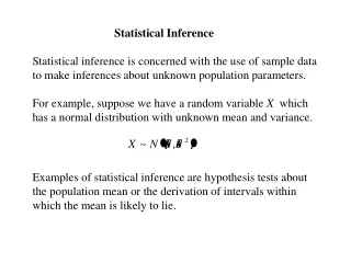
Statistical Inference and Hypothesis Testing for Means and Variances
Learn how to compare means and variances of populations using z-distribution, t-distribution, and F-distribution. Test null and alternative hypotheses with one-tailed and two-tailed tests. Make informed decisions based on significance levels.

Statistical Inference and Hypothesis Testing for Means and Variances
E N D
Presentation Transcript
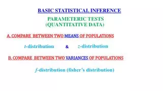
BASIC STATISTICAL INFERENCE PARAMETERIC TESTS (QUANTITATIVE DATA) A. COMPARE BETWEEN TWO MEANS OF POPULATIONS z-distribution t-distribution & B. COMPARE BETWEEN TWO VARIANCES OF POPULATIONS f-distribution (fisher’s distribution)
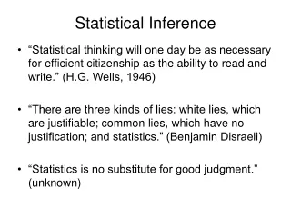
BASIC STATISTICAL INFERENCE TEST THE NULL HYPOTHESIS We shall consider here three forms for the alternative hypothesis: TEST THE ALTERNATIVE HYPOTHESIS usually represents some postulated value which needs confirmation.
One tailed test 0.05 significant level Not significant 0.95 Distribution showing 0.05 significant level in one-tailed test Insignificant difference P > 0.05 Not significant ? 0.05 significant level P < 0.05 P < 0.001 P < 0.01 0.95 Distribution showing 0.05 significant level in one-tailed test
Two tailed test 0.05 significant level 0.05 significant level Not significant 0.95 Distribution showing 0.05 significant level in two-tailed test
Calculated t Frequency 0.05 0.01 0.001 𝝈 𝝈 Tabulated t
Accept H0 Reject H0 Reject H0 P > 0.05
HYPOTHESIS TESTS ON THE MEAN (LARGE SAMPLES >30) Mean sample A given fixed value to be tested Calculated z Sample size (>30) Population standard deviation
HYPOTHESIS TESTS ON THE MEAN (SMALL SAMPLES <30) Mean sample A given fixed value to be tested Calculated z Sample size (<30) Sample standard deviation
One sample t-distribution • To decide if a sample mean is different from a hypothesized population mean. • You have calculated mean value and standard deviation for the group assuming you have measurement data. where the standard score (t) is: Degree of freedom (n-1)
t-distribution • The percentiles values of the t-distribution (tp) are tabulated for a range of values of d.f. and several values of p are represented in a Table .
One sample t-DISTRIBUTION Example The mean concentration of cadmium in water sample was 4 ppm for sample size 7 and a standard deviation=0.9 ppm. The allowable limit for this metal is 2 ppm. Test whether or notthe cadmium level in water sample at the allowable limit. Solution T cal(2.447) > t tab (2.447) Reject the null hypothesis Reject the null hypothesis T cal(2.447) > t tab (3.707) Decision: Thus the cadmium level in water is not at the allowable limit.
Two sample INDEPENDENT t-DISTRIBUTION Example: In an New Zealand, Does the average mass of male turtles in location A was significantly higher than Location B? = d.f.= n1 + n2 - 2 = 25 + 26 - 2 = 49 Tabulated t at df 59 = 1.671 Thus,tobserved (3.35) > ttabulated (1.67) at α= 0.05 The mass of male turtles in location A is significantly higher than those of location B (reject H0) P<0.05
d.f.= n1 + n2 - 2 = 11+11 -2= 20 =70.45 =60.18 tcalculated(2.209) > ttabulated(2.086) at d.f. 20
Two sample DEPENDENT t-DISTRIBUTION TESTING THE DIFFERENCE BETWEEN TWO MEANS OF DEPENDENT SAMPLES d.f. = n - 1 ? d.f. = 10 – 1= 9 ttabulated at d.f. 10 = 1.833
Fisher’s F-distribution That is, you will test the null hypothesis H0: σ12 = σ22against an appropriate alternate hypothesis Ha: σ12≠ σ22. You calculate the F-value as the ratio of the two variances: • where s12 ≥ s22, so that F ≥ 1. • The degrees of freedom for the numerator and denominator are n1-1 and n2-1, respectively. • Compare Fcalc.to a tabulated value Ftab.to see if you should accept or reject the null hypothesis.
Example: Assume we want to see if a Method 1for measuring the arsenic concentration in soil is significantly more precise than Method 2. Each method was tested ten times, with yielding the following values: Solution: So we want to test the null hypothesis H0: σ22 = σ12 against the alternate hypothesis HA: σ22 > σ12 d.f.= 10 – 1 = 9 • The tabulated value for d.f.= 9 in each case, at 1-tailed, 95% confidence level is F9,9 = 3.179. • In this case, Fcalc < F9,9 tabulated, so we Accept H0that the two standard deviations are equal,so P > 0.05 • We use a 1-tailed test in this case because the only information we are interested in is whether Method 1 is more precise than Method 2