Basic Statistical Methods
Basic Statistical Methods. Why a t-Test Isn’t Always the Answer Laura Hendrix BSc. BEd. MSc. Clinical Research Coordinator Clinical Research Consortium Department of Surgery. Don’t Believe Everything You Read!. Error rates of upwards of 50% in high-quality mainstream medical journals

Basic Statistical Methods
E N D
Presentation Transcript
Basic Statistical Methods Why a t-Test Isn’t Always the Answer Laura Hendrix BSc. BEd. MSc. Clinical Research Coordinator Clinical Research Consortium Department of Surgery
Don’t Believe Everything You Read! • Error rates of upwards of 50% in high-quality mainstream medical journals • A review of surgical journals (Annals, Archives, JACS, JSR, Surgery) from 1985-2003: 27% of studies with incorrect selection or reporting of statistical methods • A 2003 review of 70 studies published in high impact journals (NEJM,JAMA, Lancet, BMJ): 68% used only elementary summary statistics
Purpose • To give a brief overview of basic statistical methods and their use/misuse • To help you determine the most appropriate techniques for your data • To help you plan studies to facilitate statistical analyses
Why Do Statistics? • We use data from a sample of the population to make inferences about the entire population • Want to determine whether there are significant differences between groups • Need to evaluate how representative our sample data is in order to generalize results to the entire population
Normal Distribution • Population values are distributed according to the Standard Normal Distribution with mean=0 and standard deviation=1 • Eg) height distribution of UNC students • 95% of all values are within 1.96 sd of the mean • Proportions follow a similar distribution (Binomial distribution) height Number of students
Types of Data • Continuous – evaluate mean • Age, weight, number of children • Data follows Normal (binomial) distribution in populations – check your data! • Binary – evaluate proportions with/without • Death, gender • Categorical – evaluate proportions • Ordinal – age categories, Likert scale • Nominal – ethnicity • Be careful when categorizing continuous data – eg. Age -> agegroup • Think about how data will be analyzed BEFORE it is collected!
Measures of Difference • Single sample – compared to a specified value: • Proportions • Means • Two independent samples (eg. treatment vs control): • Difference in proportions • Difference in means • Test for trend • Paired samples (eg. before-and-after in same people) • Difference in proportions • Difference in means Procedure the same for all: • Calculate difference • Calculate 95% confidence interval • Test hypothesis – significance of results
Parametric vs. Nonparametric Hypothesis Tests • Hypothesis tests – evaluate whether obtained values are significant • Parametric tests (eg. t-test)– make assumptions about data • If these assumptions are violated, nonparametric methods should be used
Parametric Tests – Assumptions • Data is Normally distributed – check with histogram or compare mean & median • Equal variance in groups being compared • Independence • No clustering – test • No repeated measures – use ANOVA
Check for Normality Mean=15 Median=8 TBSA of Admissions to Burn Center >60 yrs 2000-2008
Transforming Non-Normal Data Back-transform to obtain 95% CI in original scale STATA – gladder command
Inference With a Single Mean • Take a sample of 150 UNC students and find mean height = 169.6 cm; standard deviation of 9.2 cm – how representative is this sample of all UNC students?
95% Confidence Interval • Interval around estimate derived from sample data around which we can be 95% confident contains the true population mean • More important than p-value! • wide CIs indicate small samples and/or large degree of variation in the sample – lack of precision even if p<0.05 • If null value contained within CI, p will be>0.05
Hypothesis Test • Test to determine whether sample mean is in agreement with a specified value • eg) is mean height of UNC students the same as the mean height of Duke students, 171.4 cm? • Null hypothesis (Ho): the mean height of UNC students is 171.4cm • Alternative hypothesis (Ha): the mean height is not 171.4 cm
z/t-test • For large samples (n>100) calculate a z-statistic and compare to table of z-values • Interpretation of p-value: probability of finding the mean value we did if the true population mean is really 171.4 cm = 1% • p<0.05 – reject null hypothesis; therefore the mean height of UNC students is significantly different from 171.4 cm *This can be done in Excel
P-value Warning! • Reliance on p-value to determine validity of a study can be dangerous! • Possible to get a significant result by chance (p=0.05 = 5% of the time=1 in 20) • Values near 0.05 difficult to interpret – “borderline” • Better to refer to 95% CI
Comparing Two Means/Proportions • Essentially the same method but instead of comparing to a specified value, the difference between means and proportions is evaluated • Ho: difference=0 • Different methods required for independent and paired samples
Small Sample Sizes (n<100) • Assumptions of Normality and Independence still hold but n<100 • Use t-distribution & t-test instead of z-test for hypothesis testing (as n gets larger, approaches z-distribution)
Measures of Association • 2x2 Contingency Table • Is there an association between race and flame burn? If so, how strong is the association? • Chi-squared test – compares observed and expected values in each cell • Check assumptions – eg. n>40! p=0.912
Correlation • Used to evaluate degree of association between continuous variables
Correlation • Assess Pearson’s correlation coefficient, r (-1 - +1), which describes the strength of the relationship; rule of thumb: r>0.75 • r of 0 does not always mean no relationship • Plot your data! • Check assumptions – eg. Both variables normally distributed • Linear regression – plots line of best fit (carry out diagnostics!) and allows prediction of change in y for x (multiple linear regression – evaluate for confounding)
Measures of Effect – Risk/Odds • Risk = died/total • Risk ratio = risk(whites)/risk (nonwhites) • Odds=died/survived • Odds ratio=odds(whites)/odds(nonwhites) • 95% CI and p-values • Rates/Rate ratio – include total follow up time
Measures of Effect • Calculate 95% CI • Hypothesis test Ho: OR/RR = 1 • Ratios closer to 1 indicate smaller effects • If 95% CI includes 1, p>0.05
Logistic Regression • For modeling risk and prevalence (binary outcomes) • Uses odds and odds ratios • Can adjust estimates for multiple confounding factors • Rates – use Poisson regression • Follow step by step process – don’t just plug in numbers!
Non-Parametric Methods • If sample size does not meet requirements for parametric methods these can be used • Small sample size – eg. lab experiments • Quantitative data that are not Normally distributed • Categorical variables with more than two categories • Non-parametric methods don’t require parametric assumptions about population distribution • This does not mean “assumption-free”
Non-Parametric Methods • These utilize rank of observations instead of their actual values • Compare the order rather than the size • Use median instead of mean • Disadvantage: original data is lost • Most non-parametric methods deal with hypothesis testing rather than estimation of effects
Compare values to published tables to obtain 95% CI and p-values OR use software! Median value=202 mmol/dL (mean=221 mmol/dL)
Criteria for Determining Study Size • Precision of effect measures – how wide of a CI do you want? • Power of study – probability of obtaining a statistically significant result • Power calculators widely available DETERMINE IN PLANNING PHASE! • Is it worth the resources to carry out a study that will not reach significance?
Sample Size Example – Hookworm/Anaemia • 69% anaemic • Deworming reduces by 5-10%
Size For Adequate Power 1. Select minimum difference between groups that is clinically relevant 2. Specify level of confidence of obtaining significant results if this is the true difference • Commonly used – 80, 90, 95 percent 3. Specify significance level – typically 0.05
More Tips for Study Planning • Have an a priori hypothesis – prevents accusations of “data dredging” • Multiple comparisons and subgroup analyses – risky! • Have well developed data collection instruments • Don’t use Excel for data entry! – double entry-EpiInfo • Be specific about the data you NEED (and have a reason for collecting it!) – the rest is “noise” – makes entry and analysis more efficient
Resources • UNC Biostats department • Odom Institute • Library • CONSORT guidelines http://www.consort-statement.org