Modeling in the Time Domain - State-Space
590 likes | 1.11k Vues
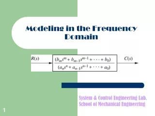
Modeling in the Time Domain - State-Space. Mathematical Models. Classical or frequency-domain technique State-Space or Modern or Time-Domain technique. Advantages Converts differential equation into algebraic equation via transfer functions.

Modeling in the Time Domain - State-Space
E N D
Presentation Transcript
Mathematical Models • Classical or frequency-domain technique • State-Space or Modern or Time-Domain technique
Advantages Converts differential equation into algebraic equation via transfer functions. Rapidly provides stability & transient response info. Disadvantages Applicable only to Linear, Time-Invariant (LTI) systems or their close approximations. Classical or Frequency-Domain Technique LTI limitation became a problem circa 1960 when space applications became important.
Advantages Provides a unified method for modeling, analyzing, and designing a wide range of systems using matrix algebra. Nonlinear, Time-Varying, Multivariable systems Disadvantages Not as intuitive as classical method. Calculations required before physical interpretation is apparent State-Space or Modern or Time-Domain Technique
State-Space Representation An LTI system is represented in state-space format by the vector-matrix differential equation (DE) as: Dynamic equation(s) Measurement equations The vectors x, y, and u are the state, output and input vectors. The matrices A, B, C, and D are the system, input, output, and feedforward matrices.
Definitions • System variables: Any variable that responds to an input or initial conditions. • State variables: The smallest set of linearly independent system variables such that the initial condition set and applied inputs completely determine the future behavior of the set. Linear Independence: A set of variables is linearly independent if none of the variables can be written as a linear combination of the others.
Definitions (continued) • State vector: An (n x 1) column vector whose elements are the state variables. • State space: The n-dimensional space whose axes are the state variables. Graphic representationof state spaceand a state vector
The minimum number of state variables is equal to: • the order of the DE’s describing the system. • the order of the denominator polynomial of its transfer function model. • the number of independent energy storage elements in the system. Remember the state variables must be linearly independent! If not, you may not be able to solve for all the other system variables, or even write the state equations.
Case Study: Pharmaceutical Drug Absorption Advantages of the state-space approach are the ability to focus on component parts of the system and to represent multiple-input, multiple-output systems.
Pharmaceutical Drug Absorption Problem We wish to describe the distribution of a drug in the body by dividing the process intocompartments: dosage, absorption site, blood, peripheral compartment, and urine. Each is the amount of drug in that particular compartment.
Pharmaceutical Drug Absorption Solution 1. Assume dosage is released at a rate proportional to concentration. 2. Assume rate of accumulation at a site is a linear function of the dosage of the donor compartment and the resident dosage. Then,
Pharmaceutical Drug Absorption Solution 3. Define the state vector as the dosage amount in each compartment and assume we measure the dosage in each compartment. Then,
Converting a Transfer Function to State Space • State variables are not unique. A system can be accurately modeled by several different sets of state variables. • Sometimes the state variables are selected because they are physically meaningful. • Sometimes because they yield mathematically tractable state equations. • Sometimes by convention.
Phase-variable Format 1. Consider the DE 2. The minimum number of state variables is n since the DE is of nth order. 3. Choose the output and its derivatives as state variables.
Phase-variable Format (continued) 4. Arrange in vector-matrix format Note the transfer function format
Example 3.4 equivalentblock diagram showingphase-variables.Note: y(t) = c(t)
Transfer Function with Numerator Polynomial (continued) 1. From the first block: 2. Therefore,
Transfer Function with Numerator Polynomial (continued) 3. The measurement (observation) equation is obtained from the second transfer function.
Converting from State Space to a Transfer Function Taking the Laplace transform,
Example 3.6 p.p.152-153 • Solve by hand • Solve using MATLAB’s ‘ss’ and ‘tf’ commands
Linearization • Demonstration of how to linearize a nonlinear state space model about a nominal solution. • Application of linearization to guidance and control of a lunar mission.