Download
1 / 24
250 likes | 404 Vues
Fast and Exact Geometric Analysis of Real Algebraic Plane Curves. Arno Eigenwillig, Michael Kerber, Nicola Wolpert. Motivation. Arrangements of arbitrary algebraic curves are missing. With the Bitstream-Descartes Method (Eigenwillig et al.`05) we now have a powerful tool.

E N D
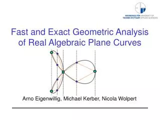
Fast and Exact Geometric Analysisof Real Algebraic Plane Curves Arno Eigenwillig, Michael Kerber, Nicola Wolpert
Motivation • Arrangements of arbitrary algebraic curves are missing. • With the Bitstream-Descartes Method (Eigenwillig et al.`05) we now have a powerful tool.
Remember: The Descartes Method Input: Squarefree polynomial p(x) Q[x].Output: Rational intervals isolating the real roots of p(x). Descartes rule of signs:# sign variations in coefficient sequence of p= # real roots of p in (0,) + 2i, i hN x
x Remember: The Descartes Method Input: Squarefree polynomial p(x) Q[x].Output: Rational intervals isolating the real roots of p(x). Descartes rule of signs:# sign variations in coefficient sequence of Tp,c,d (x)= # real roots of p in(c,d) + 2i, i N 0 sign changes # real roots of p in(c,d)= 01 sign change # real roots of p in(c,d)= 12 sign changes # real roots of p in(c,d)= 0 or2 3 sign changes # real roots of p in(c,d)= 1 or3
x Bitstream-Descartes Method Input: Squarefree polynomialp(x)= pi xiwith bit-stream coefficients. bit-stream coefficients: approximable to any precision but not known exactly, e.g. pi = algebraic numbers Output: Rational intervals isolating the real roots ofp(x).The validity of the isolating intervals is guaranteed for the exact polynomial p(x).
The Problem Input: Bivariate polynomialfwith rational coefficientsf(x,y) := 2x4+y4-x3+xy2Output: Description of the topology of the curve defined byfin the original coordinate system
The main Idea • Projection Phase: Compute x-coordinates of critical points: singular pointsx-extreme points (of arc diverging against a vertical asymptote) • Lifting Phase: - Compute stacks over critical points - and inbetween two critical points, - connect the stacks Goal: Compute the exact result!
Previous Work • Collins 1975 • Hong 1996 • Gonzalez-Vega, El Kahoui 1996 • Gonzalez-Vega, Necula 2002 • Seidel, Wolpert 2005 • and many many others ...
Usual Approach • Find x-coordinatesa1,...,anof the critical points • Find rational valuesr0<a1<r1< ...<an< rn • For eachaifind the real rootsbijoff(ai,y)+identify the critical points:Compute the stacks over the critical points • For eachrjfind the real rootscjkoff(rj,y):Compute the stacks inbetween • Connect the stacks
Usual Approach • Findx-coordinatesa1,...,anof the critical points • Find rational valuesr0<a1<r1< ...<an< rn • For eachaifind the real rootsbijoff(ai,y) + identify the critical points:Variant of the Bitstream-Descartes Method • For eachrjfind the real rootscjkoff(rj,y):Descartes Method • Connect the stacks The coefficients off(ai,y)are algebraic numbers
Usual Approach • 0. Shear coordinate system so that curve is in generic position:- no two critical points on a vertical line- no vertical asymptote- no vertical line contained in curve • Find x-coordinatesa1,...,anof the critical points • Find rational valuesr0<a1<r1< ...<an< rn • For eachaifind the real rootsbijoff(ai,y)+identify critical points:Variant of the Bitstream-Descartes Method • For eachrjfind the real rootscjkoff(rj,y) • Connect the stacks
Usual Approach • 0. Shear coordinate system so that curve is in generic position:- no two critical points on a vertical line- no vertical asymptote- no vertical line contained in curve • Find x-coordinatesa1,...,anof the critical points • Find rational valuesr0<a1<r1< ...<an< rn • For eachaifind the real rootsbijoff(ai,y)+identify critical points:Variant of the Bitstream-Descartes Method • For eachrjfind the real rootscjkoff(rj,y) • Connect the stacks • (Go back to the original coordinate system) Genericity is tested with no additional cost in Step 3.
Tool from Algebra Given a polynomialf(x,y) Q[x,y]of degree n. Computesequence of itsprincipal Sturm-Habicht coefficients: (sthan(f ),...,stha0(f )), with sthai(f) Q[x]. TheoremAfter specializationx=athe signs of(sthan(f )(a),...,stha0(f )(a))indicatek:= deg( gcd ( f (a,y), f ´(a,y) ) ), m:= #{bhR | f (a,b)=0}
Our Algorithm • Find x-coordinatesa1,...,anof critical points:Isolate the real roots ofstha0(f ) Q[x]using Descartes Method a3 a4 a1 a6 a2 a5
Our Algorithm • Find x-coordinatesa1,...,anof critical points:Isolate the real roots ofstha0(f ) Q[x]using Descartes Method • Find rational valuesr0<a1<r1< ...<an< rn a3 a4 a6 a2 a1 a5 r3 r0 r5 r2 r6 r1 r4
Our Algorithm • Find x-coordinatesa1,...,anof critical points:Isolate the real roots ofstha0(f ) Q[x]using Descartes Method • Find rational valuesr0<a1<r1< ...<an< rn • For eachaifind the real rootsbijoff(ai,y)+ identify the critical points;test genericity during execution:Variant of the Bitstream-Descartes Method a3
Our Algorithm • Find x-coordinatesa1,...,anof critical points:Isolate the real roots ofstha0(f ) Q[x]using Descartes Method • Find rational valuesr0<a1<r1< ...<an< rn • For eachaifind the real rootsbijoff(ai,y)+ identify the critical points;test genericity during execution:Variant of the Bitstream-Descartes Method • For eachrjfind the real rootscjkoff(rj,y): Descartes Method r2
Our Algorithm • Find x-coordinatesa1,...,anof critical points:Isolate the real roots ofstha0(f ) Q[x]using Descartes Method • Find rational valuesr0<a1<r1< ...<an< rn • For eachaifind the real rootsbijoff(ai,y)+identify the critical points;test genericity during execution:Variant of the Bitstream-Descartes Method • For eachrjfind the real rootscijoff(ri,y): Descartes Method • Connect the stacks • (Go back to original coordinate system) a3 a4 a6 a2 a1 a5 r3 r0 r5 r2 r1 r4
a3 m-k-Descartes Method • For eachaifind the real rootsbijoff(ai,y)+identify the critical points+ test genericity during execution • f(ai,y)not square free Bitstream Descartes not applicable directly • Compute k:= deg( gcd (f (ai,y),f ´(ai,y) ) ),(k=1)m:= #{bhR | f (ai,b)=0},(m=3) • m-k-Descartes Method: Run theBitstream Descartes on f (ai,y) until • m-1 simple roots + 1 additional interval: success case • or every interval counts k sign variations: fnot generic
Termination • Run theBitstream Descartes until • m-1 simple roots + 1 additional interval: success case • or every interval counts k sign variations: fnot generic • Lemma 1: m-k-Descartes always terminates. • Proof: • terminates for intervals with 0 or 1 root (proof for squarefree case) • f(ai,y) has 1 multiple root terminates in success case • f(ai,y) has >1 multiple root multiplicity of each root k • known: for r-fold root it terminates with r sign variations
Success Case • Run theBitstream Descartes until • m-1 simple roots + 1 additional interval: success case • or every interval counts k sign variations: fnot generic • Lemma 2:f generic m-k-Descartes succeeds • Proof:We show: Second condition never satisfied for f(ai,y).f generic f(ai,y)has at most 1 multiple root gcd (f (ai,y),f ´(ai,y) ) = (y – b)kfor some b R bis (k+1)-fold root of f(ai,y) interval for bcounts (k+1) sign variations
Connect the Stacks • e.g. Gonzalez-Vega, Necula`02 • a := # roots above critical pointb := # roots below critical point • Connect the a highest roots at x=ri / x=ri+1with the a highest roots at x=ai • Connect the b lowest roots at x=ri / x=ri+1with the b lowest roots at x=ai • Connect the remaining roots at x=ri / x=ri+1with the critical point at x=ai a3 r3 r2
Experiments • Our algorithm is implemented as the C++ library AlciX in EXACUS. • Comparisons: as proposed by the respective authors, all on the same machine • Top (Gonzales-Vega, Necula) • Insulate (Seidel, Wolpert) • Faster in each example: factor 2 - 61 • cad2d (Brown) • Competitive for any curve, superior for curves with singularities Maple
Future Work • Compute arrangements of curves • Compute the geometry of space-curves