Scheduling
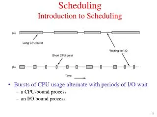
Scheduling. Alternating Sequence of CPU And I/O Bursts. Simple Categories of Processes. CPU-bound process is one that has more and larger CPU bursts (spends most of its time computing). An I/O-bound process spends most of its time waiting for I/O. . Histogram of CPU-burst Times.

Scheduling
E N D
Presentation Transcript
Simple Categories of Processes • CPU-bound process is one that has more and larger CPU bursts (spends most of its time computing). • An I/O-bound process spends most of its time waiting for I/O.
Computing Environments • Batch • E.g., supercomputing centers, mainframes/workstations for business computing.
Interactive Systems (e.g., Gandalf). • Real-Time systems.
CPU Scheduler • Selects from among the processes in memory (on ready queue), and allocates the CPU to one of them. • CPU scheduling decisions may take place when a process: 1. Switches from running to waiting state. 2.Switches from running to ready state. 3. Switches from waiting to ready. 4. Terminates. • Scheduling under 1 and 4 is nonpreemptive. • All other scheduling is preemptive.
Dispatcher • Dispatcher module gives control of the CPU to the process selected by the short-term scheduler; this involves: • switching context • switching to user mode • jumping to the proper location in the user program to restart that program • Dispatch latency – time it takes for the dispatcher to stop one process and start another running.
Possible Scheduling Goals • CPU utilization – keep the CPU as busy as possible • Throughput – # of processes that complete their execution per time unit • Turnaround time – amount of time to execute a particular process
Possible Scheduling Goals (continued) • Waiting time – amount of time a process has been waiting in the ready queue • Response time – amount of time it takes from issuing a command and getting response (interactive systems, PCs).
Optimization Criteria • Max CPU utilization • Max throughput • Min turnaround time • Min waiting time • Min response time
Optimization Criteria: Conflicting • Maximize throughput • Execute all shortest jobs first. • Minimize turnaround time • Turnaround time is increased significantly if long jobs are never executed.
Goals of Scheduling Algorithms • All systems: • Fairness • Balance (keep all parts of the system busy). • Batch Systems: • Maximize throughput. • Minimize turnaround time • CPU utilization. • Interactive systems: • Response time.
Real-time systems: • Meeting deadlines
First-Come, First-Served (FCFS) Scheduling • Allocate CPU to processes based on arrival order. • Non-preemptive. Process executes until completes or blocks on I/O or other system resource. • Not a good idea for a timesharing system!
First-Come, First-Served (FCFS) Scheduling ProcessBurst Time P1 24 P2 3 P3 3 • Suppose that the processes arrive in the order: P1 , P2 , P3
P1 P2 P3 0 24 27 30 The Gantt Chart for the schedule is: • Waiting time for P1 = 0; P2 = 24; P3 = 27 • Average waiting time: (0 + 24 + 27)/3 = 17
P2 P3 P1 0 3 6 30 FCFS Scheduling (Cont.) Suppose that the processes arrive in the order P2 , P3 , P1 . • The Gantt chart for the schedule is: • Waiting time for P1 = 6;P2 = 0; P3 = 3 • Average waiting time: (6 + 0 + 3)/3 = 3 • Much better than previous case.
One problem with FCFS is that average waiting time can be quite large. • Another problem is the Convoy effect. • Consider: • 4 processes; • 1 CPU-bound with CPU burst of 20 units followed by an I/O request requiring 10 units. • 3 I/O bound processes with 1 unit of CPU burst followed by 10 units of I/O.
0 19 20 21 22 P0 P1 P2 P3
0 19 20 21 22 P0 P1 P2 P3 I/O 1 I/O 2 I/O 3 I/O 4 P0: 7 P1: 8 P2: 9 P3: 10
I/O Devices Idle CPU Idle 0 19 20 21 22 29 P0 P1 P2 P3 P0 I/O 1 I/O 2 I/O 3 I/O 4 P1: 1 P2: 2 P3: 3
I/O Devices Idle CPU Idle I/O Devices Idle 0 19 20 21 22 29 32 49 P0 P1 P2 P3 P0 I/O 1 I/O 2 I/O 3 I/O 4
FCFS Scheduling (Cont.) • Convoy effect short I/O bound processes behind long CPU-bound process. • CPU-bound process executes, I/O processes wait in Ready Queue. • CPU-bound process completes execution burst and waits on I/O device. • IO-Bound processes quickly complete CPU burst and block on I/O device. • CPU is idle until I/O completed for CPU-bound process. • CPU-bound process resumes, I/O-bound processes complete I/O request and move to RQ. • I/O devices idle while CPU-bound process monopolizes CPU.
Shortest-Job-First(SJR) Scheduling • Associate with each process the length of its next CPU burst. Use these lengths to schedule the process with the shortest time. • Two schemes: • nonpreemptive – once CPU given to the process it cannot be preempted until completes its CPU burst.
Shortest-Job-First (SJR) Scheduling • preemptive – if a new process arrives with CPU burst length less than remaining time of current executing process, preempt. This scheme is know as the Shortest-Remaining-Time-First (SRTF). • SJF is optimal – gives minimum average waiting time for a given set of processes.
P1 P3 P2 P4 0 3 7 8 12 16 Example of Non-Preemptive SJF Process Arrival TimeBurst Time P1 0.0 7 P2 2.0 4 P3 4.0 1 P4 5.0 4
P1 P3 P2 P4 0 3 7 8 12 16 Example of Non-Preemptive SJF • Average waiting time = (0 + 6 + 3 + 7)/4 = 4
Preemptive Shortest Job First • If a job arrives at the queue with a burst time less than that of the running process, the running process is preempted. • Decision only made when a new process enters the queue.
Preemptive SJF Process Arrival Time Burst Time P1 0.0 7 P2 2.0 4 P3 4.0 1 P4 5.0 4
P1 11 16 0 2 4 5 7 Process Arrival Time Burst Time P1 0.0 7 P2 2.0 4 P3 4.0 1 P4 5.0 4
P1 P2 P3 P2 P4 P1 11 16 0 2 4 5 7 Process Arrival TimeBurst Time P1 0.0 7 P2 2.0 4 P2 Remainder = 4. P1 Remainder = 5. Result: P1 preempted at time 2.
P1 P2 P3 P2 P4 P1 11 16 0 2 4 5 7 Process Arrival TimeBurst Time P1 0.0 7 P2 2.0 4 P3 4.0 1 P1: 5 P2: 2 P2 Preempted. P3 completes at time 5. P3: 1
Process Arrival TimeBurst Time P1 0.0 7 P2 2.0 4 P4 5.0 4 P1: 5 P2: 2 P4: 4
P1 P2 P3 P2 P4 P1 11 16 0 2 4 5 7 P2 Completes at time 7. P1: Remaining time of 5. P4: Remaining time of 4.
Process Arrival Time Burst Time P1 0.0 7 P2 2.0 4 P3 4.0 1 P4 5.0 4 P1 P2 P3 P2 P4 P1 11 16 0 2 4 5 7 P1: Waits from time 2 to time 11 = 9 P2: Waits from time 4 to time 5 = 1 P3: No waiting = 0 P4: Waits from time 5 to time 7 = 2 Average wait = 12/4 = 3.
Determining Length of Next CPU Burst • Can only estimate the length. • Estimate made based on some sort of statistic of historical behavior. • Assume BL2 == BL1 (Next same as last). • Take mean of last n burst lengths. • Exponential average of previous bursts.
Homework #2 • Please answer the following question from Chapter 5. • 5.2, 5.4, 5.5, 5.6, 5.7, 5.8, 5.10, and 5.13. For problem 5.8, it should read as follows. • “... Implementing a multi-level feedback queue ........”
Scheduling in Batch Systems Three level scheduling
Memory Scheduler • Decisions based on for example: • Time since swapped out. • Amount of CPU time allocated so far. • How large. • How important.
Admission Scheduler • Based on “degree of multiprogramming” • Process mix.
Priority Scheduling • A priority number (integer) is associated with each process • The CPU is allocated to the process with the highest priority (smallest integer highest priority). • Preemptive • nonpreemptive • SJF is a priority scheduling where priority is the predicted next CPU burst time. • Problem Starvation – low priority processes may never execute.
Priority Scheduling • Solution Aging – as time progresses increase the priority of the process. • Unix has mechanism for user to lower their priority through the nice system call.
Scheduling for Interactive Systems: Round Robin (RR) • Each process gets a small unit of CPU time (time quantum), usually 10-100 milliseconds. • After this time has elapsed, the process is preempted and added to the end of the ready queue. • If there are n processes in the ready queue and the time quantum is q, then each process gets 1/n of the CPU time in chunks of at most q time units at once. • No process waits more than (n-1)q time units.
Scheduling for Interactive Systems: Round Robin (RR) • Performance • q large FIFO • q small High overhead: Must be large with respect to context switch, otherwise overhead is too high.
Scheduling in Interactive Systems • Round Robin Scheduling • a) list of runnable processes • b) list of runnable processes after B uses up its quantum
How long should the quantum be? • quantum too short • Assume switch time = 5ms and quantum = 20ms: Wasted time = 5/(5+20) = 20% • quantum too long: e.g., switch time = 5ms, quantum = 200ms: Wasted time = 5/(5+200) = approx. 2% but if have 100 processes, response time for 200th is pretty bad. This is the quantum Linux uses.