Scheduling
Scheduling. The art and science of allocating the CPU and other resources to processes (Slides include materials from Operating System Concepts , 7 th ed., by Silbershatz, Galvin, & Gagne and from Modern Operating Systems , 2 nd ed., by Tanenbaum). Why Scheduling?.

Scheduling
E N D
Presentation Transcript
Scheduling The art and science of allocating the CPU and other resources to processes (Slides include materials from Operating System Concepts, 7th ed., by Silbershatz, Galvin, & Gagne and from Modern Operating Systems, 2nd ed., by Tanenbaum) Scheduling
Why Scheduling? • We know how to switch the CPU among processes or threads, but … • How do we decide which to choose next? • Reading Assignment – Chapter 5 of Silbershatz • Especially §§5.1–5.5 Scheduling
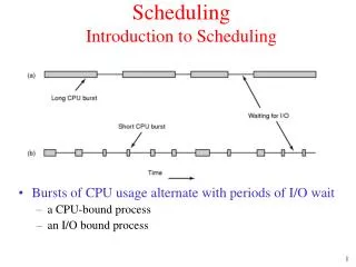
Example • Bursts of CPU usage alternate with periods of I/O wait • a CPU-bound process (a) • an I/O bound process (b) • Which process should have preferred access to CPU? • Which process should have preferred access to I/O or disk? • Why? Scheduling
Alternating Sequence of CPU And I/O Bursts Scheduling
Histogram of CPU-burst Times Scheduling
CPU Scheduler • Selects from among the processes in memory that are ready to execute, and allocates the CPU to one of them • CPU scheduling decisions may take place when a process: 1. Switches from running to waiting state 2. Switches from running to ready state 3. Switches from waiting to ready 4. Terminates • Scheduling under 1 and 4 is non-preemptive • All other scheduling is preemptive Scheduling
Dispatcher • Dispatcher module gives control of CPU to the process selected by the scheduler:– • switching context (registers, etc.) • Loading the PSW to switch to user mode and restart the selected program • Dispatch latency – time it takes for the dispatcher to stop one process and start another one running • Non-trivial in some systems Scheduling
Potential Scheduling Criteria • CPU utilization – keep the CPU as busy as possible • Throughput – # of processes that complete their execution per time unit • Turnaround time – amount of time to execute a particular process • Waiting time – amount of time process has been waiting in the ready queue • Response time – amount of time from request submission until first response is produced Scheduling
Scheduling – Policies • Issues • Fairness – don’t starve process • Priorities – most important first • Deadlines – task X must be done by time t • Optimization – e.g. throughput, response time • Reality — No universal scheduling policy • Many models • Determine what to optimize - metrics • Select an appropriate one and adjust based on experience Scheduling
Process Scheduling – System Needs Scheduling
Scheduling – Metrics • Simplicity – easy to implement • Job latency – time from start to completion • Interactive latency – time from action start to expected system response • Throughput – number of jobs completed • Utilization – keep processor and/or subset of I/O devices busy • Determinism – insure that jobs get done before some time or event • Fairness – every job makes progress Scheduling
Some Process Scheduling Strategies • First-Come, First-Served (FCFS) • Round Robin (RR) • Shortest Job First (SJF) • Variation: Shortest Completion Time First (SCTF) • Priority • Real-Time Scheduling
Scheduling Policies First Come, First Served (FCFS) • Easy to implement • Non-preemptive • I.e., no task is moved from running to ready state in favor of another one • Minimizes context switch overhead Scheduling
P1 P2 P3 0 24 27 30 Example: FCFS Scheduling ProcessBurst Time P1 24 P2 3 P3 3 • Suppose that processes arrive in the order: P1 , P2 , P3 • The time line for the schedule is:– • Waiting time for P1 = 0; P2 = 24; P3 = 27 • Average waiting time: (0 + 24 + 27)/3 = 17 Scheduling
P2 P3 P1 0 3 6 30 Example: FCFS Scheduling (continued) Suppose instead that the processes arrive in the order P2 , P3 , P1 • The time line for the schedule becomes: • Waiting time for P1 = 6;P2 = 0; P3 = 3 • Average waiting time: (6 + 0 + 3)/3 = 3 • Much better than previous case • Previous case exhibits the convoy effect: • short processes stuck behind long processes Scheduling
FCFS Scheduling (summary) • Favors compute bound jobs or tasks • Short tasks penalized • I.e., once a longer task gets the CPU, it stays in the way of a bunch of shorter task • Appearance of random or erratic behavior to users • Does not help in real situations Scheduling
Scheduling Policies – Round Robin • Round Robin (RR) • FCFS with preemption based on time limits • Ready processes given a quantum of time when scheduled • Process runs until quantum expires or until it blocks (whichever comes first) • Suitable for interactive (timesharing) systems • Setting quantum is critical for efficiency Scheduling
Round Robin (continued) • Each process gets small unit of CPU time (quantum), usually 10-100 milliseconds. • After quantum has elapsed, process is preempted and added to end of ready queue. • If n processes in ready queue and quantum = q, then each process gets 1/n of CPU time in chunks of q time units. • No process waits more than (n-1)q time units. • Performance • q large equivalent to FCFS • q small may be overwhelmed by context switches Scheduling
P1 P2 P3 P4 P1 P3 P4 P1 P3 P3 0 20 37 57 77 97 117 121 134 154 162 Example of RR with Time Quantum = 20 ProcessBurst Time P1 53 P2 17 P3 68 P4 24 • The time line is: • Typically, higher average turnaround than SJF, but better response Scheduling
Comparison of RR and FCFS Assume: 10 jobs each take 100 seconds – look at when jobs complete • FCFS – job 1: 100s, job 2: 200s, … job 10:1000s • RR • 1 sec quantum • Job 1: 991s, job 2 : 992s … • RR good for short jobs – worse for long jobs Scheduling
Application of Round Robin • Time-sharing systems • Fair sharing of limited resource • Each user gets 1/n of CPU • Useful where each user has one process to schedule • Very popular in 1970s, 1980s, and 1990s • Not appropriate for desktop systems! • One user, many processes with very different characteristics Scheduling
Shortest-Job-First (SJF) Scheduling • For each process, identify duration (i.e., length) of its next CPU burst. • Use these lengths to schedule process with shortest burst • Two schemes:– • Non-preemptive – once CPU given to the process, it is not preempted until it completes its CPU burst • Preemptive – if a new process arrives with CPU burst length less than remaining time of current executing process, preempt. • This scheme is known as the Shortest-Remaining-Time-First (SRTF) • … Scheduling
Shortest-Job-First (SJF) Scheduling (cont.) • … • SJF is provably optimal – gives minimum average waiting time for a given set of process bursts • Moving a short burst ahead of a long one reduces wait time of short process more than it lengthens wait time of long one. Scheduling
P1 P3 P2 P4 0 3 7 8 12 16 Example of Non-Preemptive SJF Process Arrival TimeBurst Time P1 0.0 7 P2 2.0 4 P3 4.0 1 P4 5.0 4 • SJF (non-preemptive) • Average waiting time = (0 + 6 + 3 + 7)/4 = 4 Scheduling
P1 P2 P3 P2 P4 P1 11 16 0 2 4 5 7 Example of Preemptive SJF Process Arrival TimeBurst Time P1 0.0 7 P2 2.0 4 P3 4.0 1 P4 5.0 4 • SJF (preemptive) • Average waiting time = (9 + 1 + 0 +2)/4 = 3 Scheduling
Determining Length of Next CPU Burst • Predict from previous bursts • exponential averaging • Let • tn = actual length of nth CPU burst • τn= predicted length of nth CPU burst • α in range 0 α 1 • Then define Scheduling
Note • This is called exponential averaging because • α = 0 history has no effect • α = 1 only most recent burst counts • Typically, α = 0.5 and τ0 is system average Scheduling
Predicted Length of the Next CPU Burst • Notice how predicted burst length lags reality • α defines how much it lags! Scheduling
Applications of SJF Scheduling • Multiple desktop windows active at once • Document editing • Background computation (e.g., Photoshop) • Print spooling & background printing • Sending & fetching e-mail • Calendar and appointment tracking • Desktop word processing (at thread level) • Keystroke input • Display output • Pagination • Spell checker Scheduling
Priority Scheduling • A priority number (integer) is associated with each process • CPU is allocated to the process with the highest priority (smallest integer highest priority) • Preemptive • nonpreemptive Scheduling
Priority Scheduling • (Usually) preemptive • Process are given priorities and ranked • Highest priority runs next • May be done with multiple queues – multilevel • SJF = priority scheduling where priority is next predicted CPU burst time • Recalculate priority – many algorithms • E.g. increase priority of I/O intensive jobs • E.g. favor processes in memory • Must still meet system goals – e.g. response time Scheduling
Priority Scheduling Issue #1 • Problem:Starvation – low priority processes may never execute • Solution: Aging – as time progresses, increase priority of waiting processes Scheduling
Priority Scheduling Issue #2 • Priority inversion • A has high priority, B has medium priority, C has lowest priority • C acquires a resource that A needs to progress • A attempts to get resource, fails and busy waits • C never runs to release resource! or • A attempts to get resources, fails and blocks • B (medium priority) enters system & hogs CPU • C never runs! • Priority scheduling can’t be naive Scheduling
Solution • Some systems increase the priority of a process/task/job to • Match level of resource or • Match level of waiting process • Some variation of this is implemented in almost all real-time operating sytems Scheduling
Priority Scheduling (conclusion) • Very useful if different kinds of tasks can be identified by level of importance • Real-time computing (later in this course) • Very irritating if used to create different classes of citizens Scheduling
Multilevel Queue • Ready queue is partitioned into separate queues: • foreground (interactive) • background (batch) • Each queue has its own scheduling algorithm • foreground – RR • background – FCFS • Scheduling must be done between the queues • Fixed priority scheduling: (i.e., serve all from foreground then from background). Possibility of starvation. • Time slice – each queue gets a certain amount of CPU time which it can schedule amongst its processes; i.e., 80% to foreground in RR • 20% to background in FCFS Scheduling
Multilevel Queue Scheduling Scheduling
Multilevel Feedback Queue • A process can move between the various queues; aging can be implemented this way • Multilevel-feedback-queue scheduler defined by the following parameters: • number of queues • scheduling algorithms for each queue • method used to determine when to upgrade a process • method used to determine when to demote a process • method used to determine which queue a process will enter when that process needs service Scheduling
Example of Multilevel Feedback Queue • Three queues: • Q0 – RR with time quantum 8 milliseconds • Q1 – RR time quantum 16 milliseconds • Q2 – FCFS • Scheduling • New job enters queue Q0 (FCFS). When it gains CPU, job receives 8 milliseconds. If it does not finish in 8 milliseconds, job is moved to queue Q1. • At Q1 job is again served FCFS and receives 16 additional milliseconds. If it still does not complete, it is preempted and moved to queue Q2. Scheduling
Multilevel Feedback Queues Scheduling
Thread Scheduling • Local Scheduling – How the threads library decides which user thread to run next within the process • Global Scheduling – How the kernel decides which kernel thread to run next Scheduling
Scheduling – Examples • Unix – multilevel - many policies and many policy changes over time • Linux – multilevel with 3 major levels • Realtime FIFO • Realtime round robin • Timesharing • Win/NT – multilevel • Threads scheduled – fibers not visible to scheduler • Jobs – groups of processes are given quotas that contribute to priorities Scheduling
Reading Assignments • Silbershatz, Chapter 5: CPU Scheduling • §5.1-5.6 • Love, Chapter 4, Process Scheduling • Esp. pp. 47-50 • Much overlap between the two • Silbershatz tends to be broader overview • Love tend to be more practical about Linux Scheduling
Instructive Example • O(1) scheduling in Linux kernel • Supports 140 priority levels • Derived from nice level and previous bursts • No queue searching • Next ready task identified in constant time • Depends upon hardware instruction to find first bit in bit array. • See Love, p. 47 Scheduling
Scheduling – Summary • General theme – what is the “best way” to run n processes on k resources? ( k < n) • Conflicting Objectives – no one “best way” • Latency vs. throughput • Speed vs. fairness • Incomplete knowledge • E.g. – does user know how long a job will take • Real world limitations • E.g. context switching takes CPU time • Job loads are unpredictable Scheduling
Scheduling – Summary (continued) • Bottom line – scheduling is hard! • Know the models • Adjust based upon system experience • Dynamically adjust based on execution patterns Scheduling
Questions? Scheduling