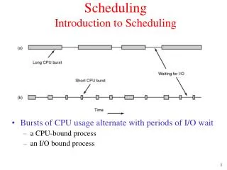
Scheduling
Scheduling. An Engineering Approach to Computer Networking. Outline. What is scheduling Why we need it Requirements of a scheduling discipline Fundamental choices Scheduling best effort connections Scheduling guaranteed-service connections Packet drop strategies. Scheduling.

Scheduling
E N D
Presentation Transcript
Scheduling An Engineering Approach to Computer Networking
Outline • What is scheduling • Why we need it • Requirements of a scheduling discipline • Fundamental choices • Scheduling best effort connections • Scheduling guaranteed-service connections • Packet drop strategies
Scheduling • Sharing always results in contention • A scheduling discipline resolves contention: • who’s next? • Key to fairly sharing resources and providing performance guarantees
Components • A scheduling discipline does two things: • decides service order • manages queue of service requests • Example: • consider queries awaiting web server • scheduling discipline decides service order • and also if some query should be ignored
Where? • Anywhere where contention may occur • At every layer of protocol stack • Usually studied at network layer, at output queues of switches
Outline • What is scheduling • Why we need it • Requirements of a scheduling discipline • Fundamental choices • Scheduling best effort connections • Scheduling guaranteed-service connections • Packet drop strategies
Why do we need one? • Because future applications need it • We expect two types of future applications • best-effort (adaptive, non-real time) • e.g. email, some types of file transfer • guaranteed service (non-adaptive, real time) • e.g. packet voice, interactive video, stock quotes
What can scheduling disciplines do? • Give different users different qualities of service • Example of passengers waiting to board a plane • early boarders spend less time waiting • bumped off passengers are ‘lost’! • Scheduling disciplines can allocate • bandwidth • delay • loss • They also determine how fair the network is
Outline • What is scheduling • Why we need it • Requirements of a scheduling discipline • Fundamental choices • Scheduling best effort connections • Scheduling guaranteed-service connections • Packet drop strategies
Requirements • An ideal scheduling discipline • is easy to implement • is fair • provides performance bounds • allows easy admission control decisions • to decide whether a new flow can be allowed
Requirements: 1. Ease of implementation • Scheduling discipline has to make a decision once every few microseconds! • Should be implementable in a few instructions or hardware • for hardware: critical constraint is VLSI space • Work per packet should scale less than linearly with number of active connections
Requirements: 2. Fairness • Scheduling discipline allocates a resource • An allocation is fair if it satisfies min-max fairness • Intuitively • each connection gets no more than what it wants • the excess, if any, is equally shared Transfer half of excess Unsatisfied demand A B A B C C
Fairness (contd.) • Fairness is intuitively a good idea • But it also provides protection • traffic hogs cannot overrun others • automatically builds firewalls around heavy users • Fairness is a global objective, but scheduling is local • Each endpoint must restrict its flow to the smallest fair allocation • Dynamics + delay => global fairness may never be achieved
Requirements: 3. Performance bounds • What is it? • A way to obtain a desired level of service • Can be deterministic or statistical • Common parameters are • bandwidth • delay • delay-jitter • loss
Bandwidth • Specified as minimum bandwidth measured over a prespecified interval • E.g. > 5Mbps over intervals of > 1 sec • Meaningless without an interval! • Can be a bound on average (sustained) rate or peak rate • Peak is measured over a ‘small’ inteval • Average is asymptote as intervals increase without bound
Delay and delay-jitter • Bound on some parameter of the delay distribution curve
Req’ments: 4. Ease of admission control • Admission control needed to provide QoS • Overloaded resource cannot guarantee performance • Choice of scheduling discipline affects ease of admission control algorithm
Outline • What is scheduling • Why we need it • Requirements of a scheduling discipline • Fundamental choices • Scheduling best effort connections • Scheduling guaranteed-service connections • Packet drop strategies
Fundamental choices 1. Number of priority levels 2. Work-conserving vs. non-work-conserving 3. Degree of aggregation 4. Service order within a level
Choices: 1. Priority • Packet is served from a given priority level only if no packets exist at higher levels (multilevel priority with exhaustive service) • Highest level gets lowest delay • Watch out for starvation! • Usually map priority levels to delay classes Low bandwidth urgent messages Realtime Non-realtime Priority
Choices: 2. Work conserving vs. non-work-conserving • Work conserving discipline is never idle when packets await service • Why bother with non-work conserving?
Non-work-conserving disciplines • Key conceptual idea: delay packet till eligible • Reduces delay-jitter => fewer buffers in network • How to choose eligibility time? • rate-jitter regulator • bounds maximum outgoing rate • delay-jitter regulator • compensates for variable delay at previous hop
Do we need non-work-conservation? • Can remove delay-jitter at an endpoint instead • but also reduces size of switch buffers… • Increases mean delay • not a problem for playback applications • Wastes bandwidth • can serve best-effort packets instead • Always punishes a misbehaving source • can’t have it both ways • Bottom line: not too bad, implementation cost may be the biggest problem
Choices: 3. Degree of aggregation • More aggregation • less state • cheaper • smaller VLSI • less to advertise • BUT: less individualization • Solution • aggregate to a class, members of class have same performance requirement • no protection within class
Choices: 4. Service within a priority level • In order of arrival (FCFS) or in order of a service tag • Service tags => can arbitrarily reorder queue • Need to sort queue, which can be expensive • FCFS • bandwidth hogs win (no protection) • no guarantee on delays • Service tags • with appropriate choice, both protection and delay bounds possible
Outline • What is scheduling • Why we need it • Requirements of a scheduling discipline • Fundamental choices • Scheduling best effort connections • Scheduling guaranteed-service connections • Packet drop strategies
Scheduling best-effort connections • Main requirement is fairness • Achievable using Generalized processor sharing (GPS) • Visit each non-empty queue in turn • Serve infinitesimal from each • Why is this fair? • How can we give weights to connections?
More on GPS • GPS is unimplementable! • we cannot serve infinitesimals, only packets • No packet discipline can be as fair as GPS • while a packet is being served, we are unfair to others • Degree of unfairness can be bounded • Define: work(I,a,b) = # bits transmitted for connection I in time [a,b] • Absolute fairness bound for discipline S • Max (work_GPS(I,a,b) - work_S(I, a,b)) • Relative fairness bound for discipline S • Max (work_S(I,a,b) - work_S(J,a,b))
What next? • We can’t implement GPS • So, lets see how to emulate it • We want to be as fair as possible • But also have an efficient implementation
Weighted round robin • Serve a packet from each non-empty queue in turn • Unfair if packets are of different length or weights are not equal • Different weights, fixed packet size • serve more than one packet per visit, after normalizing to obtain integer weights • Different weights, variable size packets • normalize weights by meanpacket size • e.g. weights {0.5, 0.75, 1.0}, mean packet sizes {50, 500, 1500} • normalize weights: {0.5/50, 0.75/500, 1.0/1500} = { 0.01, 0.0015, 0.000666}, normalize again {60, 9, 4}
Problems with Weighted Round Robin • With variable size packets and different weights, need to know mean packet size in advance • Can be unfair for long periods of time • E.g. • T3 trunk with 500 connections, each connection has mean packet length 500 bytes, 250 with weight 1, 250 with weight 10 • Each packet takes 500 * 8/45 Mbps = 88.8 microseconds • Round time =2750 * 88.8 = 244.2 ms
Weighted Fair Queueing (WFQ) • Deals better with variable size packets and weights • GPS is fairest discipline • Find the finish time of a packet, had we been doing GPS • Then serve packets in order of their finish times
WFQ: first cut • Suppose, in each round, the server served one bit from each active connection • Round number is the number of rounds already completed • can be fractional • If a packet of length p arrives to an empty queue when the round number is R, it will complete service when the round number is R + p => finish number is R + p • independent of the number of other connections! • If a packet arrives to a non-empty queue, and the previous packet has a finish number of f, then the packet’s finish number is f+p • Serve packets in order of finish numbers
A catch • A queue may need to be considered non-empty even if it has no packets in it • e.g. packets of length 1 from connections A and B, on a link of speed 1 bit/sec • at time 1, packet from A served, round number = 0.5 • A has no packets in its queue, yet should be considered non-empty, because a packet arriving to it at time 1 should have finish number 1+ p • A connection is active if the last packet served from it, or in its queue, has a finish number greater than the current round number
WFQ continued • To sum up, assuming we know the current round number R • Finish number of packet of length p • if arriving to active connection = previous finish number + p • if arriving to an inactive connection = R + p • (How should we deal with weights?) • To implement, we need to know two things: • is connection active? • if not, what is the current round number? • Answer to both questions depends on computing the current round number (why?)
WFQ: computing the round number • Naively: round number = number of rounds of service completed so far • what if a server has not served all connections in a round? • what if new conversations join in halfway through a round? • Redefine round number as a real-valued variable that increases at a rate inversely proportional to the number of currently active connections • this takes care of both problems (why?) • With this change, WFQ emulates GPS instead of bit-by-bit RR
Problem: iterated deletion • A sever recomputes round number on each packet arrival • At any recomputation, the number of conversations can go up at most by one, but can go down to zero • => overestimation • Trick • use previous count to compute round number • if this makes some conversation inactive, recompute • repeat until no conversations become inactive # active conversations Round number
WFQ implementation • On packet arrival: • use source + destination address (or VCI) to classify it and look up finish number of last packet served (or waiting to be served) • recompute round number • compute finish number • insert in priority queue sorted by finish numbers • if no space, drop the packet with largest finish number • On service completion • select the packet with the lowest finish number
Analysis • Unweighted case: • if GPS has served x bits from connection A by time t • WFQ would have served at least x - P bits, where P is the largest possible packet in the network • WFQ could send more than GPS would => absolute fairness bound > P • To reduce bound, choose smallest finish number only among packets that have started service in the corresponding GPS system (WF2Q) • requires a regulator to determine eligible packets
Evaluation • Pros • like GPS, it provides protection • can obtain worst-case end-to-end delay bound • gives users incentive to use intelligent flow control (and also provides rate information implicitly) • Cons • needs per-connection state • iterated deletion is complicated • requires a priority queue
Outline • What is scheduling • Why we need it • Requirements of a scheduling discipline • Fundamental choices • Scheduling best effort connections • Scheduling guaranteed-service connections • Packet drop strategies
Scheduling guaranteed-service connections • With best-effort connections, goal is fairness • With guaranteed-service connections • what performance guarantees are achievable? • how easy is admission control? • We now study some scheduling disciplines that provide performance guarantees
WFQ • Turns out that WFQ also provides performance guarantees • Bandwidth bound • ratio of weights * link capacity • e.g. connections with weights 1, 2, 7; link capacity 10 • connections get at least 1, 2, 7 units of b/w each • End-to-end delay bound • assumes that the connection doesn’t send ‘too much’ (otherwise its packets will be stuck in queues) • more precisely, connection should be leaky-bucket regulated • # bits sent in time [t1, t2] <= (t2 - t1) +
Parekh-Gallager theorem • Let a connection be allocated weights at each WFQ scheduler along its path, so that the least bandwidth it is allocated is g • Let it be leaky-bucket regulated such that # bits sent in time [t1, t2] <= (t2 - t1) + • Let the connection pass through K schedulers, where the kth scheduler has a rate r(k) • Let the largest packet allowed in the network be P
Significance • Theorem shows that WFQ can provide end-to-end delay bounds • So WFQ provides both fairness and performance guarantees • Boud holds regardless of cross traffic behavior • Can be generalized for networks where schedulers are variants of WFQ, and the link service rate changes over time
Problems • To get a delay bound, need to pick g • the lower the delay bounds, the larger g needs to be • large g => exclusion of more competitors from link • g can be very large, in some cases 80 times the peak rate! • Sources must be leaky-bucket regulated • but choosing leaky-bucket parameters is problematic • WFQ couples delay and bandwidth allocations • low delay requires allocating more bandwidth • wastes bandwidth for low-bandwidth low-delay sources
Delay-Earliest Due Date • Earliest-due-date: packet with earliest deadline selected • Delay-EDD prescribes how to assign deadlines to packets • A source is required to send slower than its peak rate • Bandwidth at scheduler reserved at peak rate • Deadline = expected arrival time + delay bound • If a source sends faster than contract, delay bound will not apply • Each packet gets a hard delay bound • Delay bound is independent of bandwidth requirement • but reservation is at a connection’s peak rate • Implementation requires per-connection state and a priority queue
Rate-controlled scheduling • A class of disciplines • two components: regulator and scheduler • incoming packets are placed in regulator where they wait to become eligible • then they are put in the scheduler • Regulator shapes the traffic, scheduler provides performance guarantees
Examples • Recall • rate-jitter regulator • bounds maximum outgoing rate • delay-jitter regulator • compensates for variable delay at previous hop • Rate-jitter regulator + FIFO • similar to Delay-EDD (what is the difference?) • Rate-jitter regulator + multi-priority FIFO • gives both bandwidth and delay guarantees (RCSP) • Delay-jitter regulator + EDD • gives bandwidth, delay,and delay-jitter bounds (Jitter-EDD)
Analysis • First regulator on path monitors and regulates traffic => bandwidth bound • End-to-end delay bound • delay-jitter regulator • reconstructs traffic => end-to-end delay is fixed (= worst-case delay at each hop) • rate-jitter regulator • partially reconstructs traffic • can show that end-to-end delay bound is smaller than (sum of delay bound at each hop + delay at first hop)