Graph Algorithms
Graph Algorithms. Data-Intensive Information Processing Applications ― Session #5. Jimmy Lin University of Maryland Tuesday, March 2, 2010.

Graph Algorithms
E N D
Presentation Transcript
Graph Algorithms Data-Intensive Information Processing Applications ― Session #5 Jimmy Lin University of Maryland Tuesday, March 2, 2010 This work is licensed under a Creative Commons Attribution-Noncommercial-Share Alike 3.0 United StatesSee http://creativecommons.org/licenses/by-nc-sa/3.0/us/ for details
Today’s Agenda Graph problems and representations Parallel breadth-first search PageRank
What’s a graph? • G = (V,E), where • V represents the set of vertices (nodes) • E represents the set of edges (links) • Both vertices and edges may contain additional information • Different types of graphs: • Directed vs. undirected edges • Presence or absence of cycles • Graphs are everywhere: • Hyperlink structure of the Web • Physical structure of computers on the Internet • Interstate highway system • Social networks
Some Graph Problems • Finding shortest paths • Routing Internet traffic and UPS trucks • Finding minimum spanning trees • Telco laying down fiber • Finding Max Flow • Airline scheduling • Identify “special” nodes and communities • Breaking up terrorist cells, spread of avian flu • Bipartite matching • Monster.com, Match.com • And of course... PageRank
Graphs and MapReduce • Graph algorithms typically involve: • Performing computations at each node: based on node features, edge features, and local link structure • Propagating computations: “traversing” the graph • Key questions: • How do you represent graph data in MapReduce? • How do you traverse a graph in MapReduce?
Representing Graphs • G = (V, E) • Two common representations • Adjacency matrix • Adjacency list
Adjacency Matrices Represent a graph as an n x n square matrix M • n = |V| • Mij = 1 means a link from node i to j 2 1 3 4
Adjacency Matrices: Critique • Advantages: • Amenable to mathematical manipulation • Iteration over rows and columns corresponds to computations on outlinks and inlinks • Disadvantages: • Lots of zeros for sparse matrices • Lots of wasted space
Adjacency Lists 1: 2, 4 2: 1, 3, 4 3: 1 4: 1, 3 Take adjacency matrices… and throw away all the zeros
Adjacency Lists: Critique • Advantages: • Much more compact representation • Easy to compute over outlinks • Disadvantages: • Much more difficult to compute over inlinks
Single Source Shortest Path • Problem: find shortest path from a source node to one or more target nodes • Shortest might also mean lowest weight or cost • First, a refresher: Dijkstra’s Algorithm
Dijkstra’s Algorithm Example 1 10 0 9 2 3 4 6 7 5 2 Example from CLR
Dijkstra’s Algorithm Example 10 1 10 0 9 2 3 4 6 7 5 5 2 Example from CLR
Dijkstra’s Algorithm Example 8 14 1 10 0 9 2 3 4 6 7 5 5 7 2 Example from CLR
Dijkstra’s Algorithm Example 8 13 1 10 0 9 2 3 4 6 7 5 5 7 2 Example from CLR
Dijkstra’s Algorithm Example 8 9 1 1 10 0 9 2 3 4 6 7 5 5 7 2 Example from CLR
Dijkstra’s Algorithm Example 8 9 1 10 0 9 2 3 4 6 7 5 5 7 2 Example from CLR
Single Source Shortest Path • Problem: find shortest path from a source node to one or more target nodes • Shortest might also mean lowest weight or cost • Single processor machine: Dijkstra’s Algorithm • MapReduce: parallel Breadth-First Search (BFS)
Finding the Shortest Path d1 m1 … d2 s n … m2 … d3 • m3 • Consider simple case of equal edge weights • Solution to the problem can be defined inductively • Here’s the intuition: • Define: b is reachable from a if b is on adjacency list of a • DistanceTo(s) = 0 • For all nodes p reachable from s, DistanceTo(p) = 1 • For all nodes n reachable from some other set of nodes M, DistanceTo(n) = 1 + min(DistanceTo(m), mM)
Visualizing Parallel BFS n7 n0 n1 n2 n3 n6 n5 n4 n8 n9
From Intuition to Algorithm • Data representation: • Key: node n • Value: d (distance from start), adjacency list (list of nodes reachable from n) • Initialization: for all nodes except for start node, d = • Mapper: • m adjacency list: emit (m, d + 1) • Sort/Shuffle • Groups distances by reachable nodes • Reducer: • Selects minimum distance path for each reachable node • Additional bookkeeping needed to keep track of actual path
Multiple Iterations Needed • Each MapReduce iteration advances the “known frontier” by one hop • Subsequent iterations include more and more reachable nodes as frontier expands • Multiple iterations are needed to explore entire graph • Preserving graph structure: • Problem: Where did the adjacency list go? • Solution: mapper emits (n, adjacency list) as well
Stopping Criterion • How many iterations are needed in parallel BFS (equal edge weight case)? • Convince yourself: when a node is first “discovered”, we’ve found the shortest path • Now answer the question... • Six degrees of separation? • Practicalities of implementation in MapReduce
Comparison to Dijkstra • Dijkstra’s algorithm is more efficient • At any step it only pursues edges from the minimum-cost path inside the frontier • MapReduce explores all paths in parallel • Lots of “waste” • Useful work is only done at the “frontier” • Why can’t we do better using MapReduce?
Weighted Edges • Now add positive weights to the edges • Why can’t edge weights be negative? • Simple change: adjacency list now includes a weight w for each edge • In mapper, emit (m, d + wp) instead of (m, d + 1) for each node m • That’s it?
Stopping Criterion Not true! How many iterations are needed in parallel BFS (positive edge weight case)? Convince yourself: when a node is first “discovered”, we’ve found the shortest path
Additional Complexities 1 search frontier 1 1 n6 n7 n8 10 r n9 1 n5 n1 1 1 s q p n4 1 1 n2 n3
Stopping Criterion How many iterations are needed in parallel BFS (positive edge weight case)? Practicalities of implementation in MapReduce
Graphs and MapReduce • Graph algorithms typically involve: • Performing computations at each node: based on node features, edge features, and local link structure • Propagating computations: “traversing” the graph • Generic recipe: • Represent graphs as adjacency lists • Perform local computations in mapper • Pass along partial results via outlinks, keyed by destination node • Perform aggregation in reducer on inlinks to a node • Iterate until convergence: controlled by external “driver” • Don’t forget to pass the graph structure between iterations
Random Walks Over the Web • Random surfer model: • User starts at a random Web page • User randomly clicks on links, surfing from page to page • PageRank • Characterizes the amount of time spent on any given page • Mathematically, a probability distribution over pages • PageRank captures notions of page importance • Correspondence to human intuition? • One of thousands of features used in web search • Note: query-independent
PageRank: Defined Given page x with inlinkst1…tn, where • C(t) is the out-degree of t • is probability of random jump • N is the total number of nodes in the graph t1 X t2 … tn
Computing PageRank • Properties of PageRank • Can be computed iteratively • Effects at each iteration are local • Sketch of algorithm: • Start with seed PRi values • Each page distributes PRi “credit” to all pages it links to • Each target page adds up “credit” from multiple in-bound links to compute PRi+1 • Iterate until values converge
Simplified PageRank • First, tackle the simple case: • No random jump factor • No dangling links • Then, factor in these complexities… • Why do we need the random jump? • Where do dangling links come from?
Sample PageRank Iteration (1) Iteration 1 n2 (0.2) n2 (0.166) 0.1 n1 (0.2) 0.1 0.1 n1 (0.066) 0.1 0.066 0.066 0.066 n5 (0.2) n5 (0.3) n3 (0.2) n3 (0.166) 0.2 0.2 n4 (0.2) n4 (0.3)
Sample PageRank Iteration (2) Iteration 2 n2 (0.166) n2 (0.133) 0.033 0.083 n1 (0.066) 0.083 n1 (0.1) 0.033 0.1 0.1 0.1 n5 (0.3) n5 (0.383) n3 (0.166) n3 (0.183) 0.3 0.166 n4 (0.3) n4 (0.2)
PageRank in MapReduce Map n2 n4 n3 n5 n4 n5 n1 n2 n3 n1 n2 n2 n3 n3 n4 n4 n5 n5 Reduce
Complete PageRank • Two additional complexities • What is the proper treatment of dangling nodes? • How do we factor in the random jump factor? • Solution: • Second pass to redistribute “missing PageRank mass” and account for random jumps • p is PageRank value from before, p' is updated PageRank value • |G| is the number of nodes in the graph • m is the missing PageRank mass
PageRank Convergence • Alternative convergence criteria • Iterate until PageRank values don’t change • Iterate until PageRank rankings don’t change • Fixed number of iterations • Convergence for web graphs?
Beyond PageRank • Link structure is important for web search • PageRank is one of many link-based features: HITS, SALSA, etc. • One of many thousands of features used in ranking… • Adversarial nature of web search • Link spamming • Spider traps • Keyword stuffing • …
Efficient Graph Algorithms Sparse vs. dense graphs Graph topologies
Power Laws are everywhere! Figure from: Newman, M. E. J. (2005) “Power laws, Pareto distributions and Zipf's law.” Contemporary Physics 46:323–351.
Local Aggregation • Use combiners! • In-mapper combining design pattern also applicable • Maximize opportunities for local aggregation • Simple tricks: sorting the dataset in specific ways
Questions? Source: Wikipedia (Japanese rock garden)
MapReduce and databases Data-Intensive Information Processing Applications ― Session #7 Jimmy Lin University of Maryland Tuesday, March 23, 2010 This work is licensed under a Creative Commons Attribution-Noncommercial-Share Alike 3.0 United StatesSee http://creativecommons.org/licenses/by-nc-sa/3.0/us/ for details


