Download
1 / 19
200 likes | 346 Vues
German Aerospace Center Berlin. Thermodynamics of Planetary Interiors, www.dlr.de/pf. 3D spherical gridding based on equidistant , constant volume cells for FV/FD methods. A new method using natural neighbor Voronoi cells distributed by spiral functions. German Aerospace Center Berlin.

E N D
German Aerospace Center Berlin Thermodynamics of Planetary Interiors, www.dlr.de/pf 3D spherical gridding based on equidistant, constant volume cells for FV/FD methods A new method using natural neighbor Voronoi cells distributed by spiral functions
German Aerospace Center Berlin Thermodynamics of Planetary Interiors, www.dlr.de/pf Introduction to common 3D spherical grids Most grids base on triangulated platonic solids (convex polyhedra such as the cube, dodecahedron, tetrahedron, icosahedron,...) Domain decomposition through subdivisions of the platonic solids areas Grids extend radial through a projection of the grid from the center to shells Only axisymmetric alignment; could lead to increased numerical instabilities (oscillation) Non-uniform cell size requires additional expensive compensation computations and leads to higher inner shell resolution, which is not desired in most cases (surface resolution matters!) Only fixed resolution steps (TERRA) Solve these problems through new ditribution method? TERRA grid setup and shell extension based on icosaeder subdivisions(Baumgardner, 1988)
German Aerospace Center Berlin Thermodynamics of Planetary Interiors, www.dlr.de/pf Basic Equations: In 2D cartesian coordinates: Archimede‘s Spiral: Spherical representation in 3D cartesian coordinates:
German Aerospace Center Berlin Thermodynamics of Planetary Interiors, www.dlr.de/pf The arc length equations - Non analytically inversible already! General arc length definition for 3D curves: Archimede‘s spiral (polar) arc length: Second, incomplete elliptic integral: Arc length for spherical spiral:
German Aerospace Center Berlin Thermodynamics of Planetary Interiors, www.dlr.de/pf Equidistant point distribution over the arc length Arc length for spherical spiral -We are interested in α for specific lengths s (s[i] = Resolution * i), which leads to an inversion of a non-analytically solvable integral ↷Computational expensive calculations But: Easy parallel distribution possible Equiangular > Equidistant
German Aerospace Center Berlin Thermodynamics of Planetary Interiors, www.dlr.de/pf Radial extension of the spiral sphere -Shell generation through radial re-computation (not projection!) of the new shell for the desired resolution -Shell count and overall point count is a result of inner radius, outer radius and desired resolution: • Boundary shells added before inner and after outer shell • Results in equidistant point distribution within a spherical region • „Overturning“ of the spherical spiral function leads to better distribution Comparison of the TERRA grid to the spiral grid (Surface resolution = 130km, Earth mantle): TERRA: 1,4M Points Spiral: 923.000 Points 32 Shells 32 Shells
German Aerospace Center Berlin Thermodynamics of Planetary Interiors, www.dlr.de/pf The dampening factor • Required for an optimal equidistant distribution • Used as factor for the resolution to calculate the radial shell distance and αmax • Dampening factor is optimal if the mean length of all connections of a Delauney triangulation equals the desired resolution Spiral sphere sideview d * res
German Aerospace Center Berlin Thermodynamics of Planetary Interiors, www.dlr.de/pf The influence of the dampening factor on distance
German Aerospace Center Berlin Thermodynamics of Planetary Interiors, www.dlr.de/pf Cell generation • Two methods: • Projection of a 2D spherical Voronoi tessellation of every generated shell from the sphere center; leads to a non-uniform but axisymmetric grid! • Complete 3D Voronoi tessellation • -Natural neighbor Voronoi cells lead to increased accuracy of the model 2D spherical Voronoi diagram One shell of a complete Voronoi d.
German Aerospace Center Berlin Thermodynamics of Planetary Interiors, www.dlr.de/pf Cell generation – complete 3D Voronoi diagram • Outer shell points remain as open cells and inner shell points would connect throughout the center, but both can be used as boundary zones Cut through the two-sphere in positive domain; Inner radius = 1 Outer radius = 2 Resolution = 0.1 Shells = 12 (+ 2 boundary) Points (complete): 62529
German Aerospace Center Berlin Thermodynamics of Planetary Interiors, www.dlr.de/pf Cell generation option – Centroidal Shift (CVD) • Generator points are not necessarily the center of the cell • Optional shift of generator points (from spiral) towards the center of mass of the cell • Lloyd’s algorithm iterates until the generator points reach the center point within a given criteria • Requires recomputation of Voronoi diagram on each iteration • Smoothes cell properties, but not volumes Example of Lloyd’s algorithm in 2D, random generator- point distribution CVDs do not necessarily tend to equally sized cells!
German Aerospace Center Berlin Thermodynamics of Planetary Interiors, www.dlr.de/pf Statistical analysis – Distance histogram min = 0.0733 mean = 0.0999 max = 0.1435 σ = 0.01476 skew = 0.104 min = 0.0716 mean = 0.0977 max = 0.1383σ= 0.01148 skew = 0.779
German Aerospace Center Berlin Thermodynamics of Planetary Interiors, www.dlr.de/pf Statistical analysis – Face histogram min = 10 mean = 14.513 max = 20 σ = 0.93145 skew = 0.381 min = 9 mean = 14.126 max = 19 σ= 0.85666 skew = 0.156
German Aerospace Center Berlin Thermodynamics of Planetary Interiors, www.dlr.de/pf Statistical analysis – Volume histogram min = 5.0747e-4 mean = 5.6241e-4 max = 6.14050e-4 σ = 6.7013e-6 skew = 0.111 min = 4.4102e-4 mean = 5.6271e-4 max = 6.58129e-4 σ= 1.8974e-5 skew = -0.436
German Aerospace Center Berlin Thermodynamics of Planetary Interiors, www.dlr.de/pf Statistical analysis – Volume distribution
German Aerospace Center Berlin Thermodynamics of Planetary Interiors, www.dlr.de/pf Statistical analysis – Volume distribution
German Aerospace Center Berlin Thermodynamics of Planetary Interiors, www.dlr.de/pf Possible domain decomposition for parallelization • Cones used to split the sphere into N even regions with an equivalent amount of cells • Halo zone is defined by all cells that get cut through the cone plus their natural neighbors for interpolation • Works with any even CPU counts • Zone cutting and grid information can be cached • Numbering system makes parallelization easy: One dimensional count from north-pole to south-pole, halo zones could be defined by only two numbers; complete sphere fits into 2D array: [Shell_Index, Point_Index]
German Aerospace Center Berlin Thermodynamics of Planetary Interiors, www.dlr.de/pf The diffusion equation discretized • A scalar quantity diffuses through space with a rate of • Area between cells act as energy distribution ratio to complete cell area Cell surrounded by its 13 of 14 neighbors
German Aerospace Center Berlin Thermodynamics of Planetary Interiors, www.dlr.de/pf Summary • Reliable, almost constant resolution throughout the sphere • Free choice of resolution (and therefore grid points) • Efficient parallelization through cone subdivisions • Cell volume is almost constant • Accurate diffusion through natural neighbors • No oscillation effects