Digital Data Sources Chapter 7

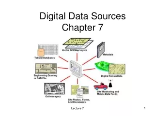
1. Digital Data SourcesChapter 7 Lecture 7

2. Introduction • Data – measurements and observations • Data quality – a measure of the fitness for use of data for a particular task (Chrisman, 1994). • Metadata – data about the data • Coordinate system & datum • Extent • Timeliness • Accuracy • Availability for use Lecture 7

3. Existing GIS Data By U.S. law, any data collected with government money must be made available to the public for free, or cost of reproduction. This is NOT true in other countries where the data is viewed as a source of income. It is the responsibility of the GIS user to determine the “fitness of use” of the data for his/her purposes. Check the metadata! Lecture 7

4. Map Services vs Locally Stored • Some data is available for transfer to, storage on, and manipulation in a local computer. • Other data are available as a Web service. • Web Mapping Service (WMS) – this is the most common form • Web Coverage Service (WCS) • Web Feature Service (WFS) Lecture 7

5. Web Mapping Service • A Web Map Service (WMS) is a standard protocol for serving (over the Internet) georeferenced map images which a map server generates using data from a GIS database. • The Open Geospatial Consortium developed the specification and first published it in 1999. https://en.wikipedia.org/wiki/Web_Map_Service Lecture 7

6. Web Coverage Service • A WCS provides access to coverage data in forms that are useful for client-side rendering, as input into scientific models, and for other clients. • WCS format encodings allow to deliver coverages in various data formats, such as GML, GeoTIFF, HDF-EOS, CF-netCDF or NITF. https://en.wikipedia.org/wiki/Web_Coverage_Service Lecture 7

7. Web Feature Service In computing, the Open Geospatial ConsortiumWeb Feature Service Interface Standard (WFS) provides an interface allowing requests for geographical features across the web using platform-independent calls. https://en.wikipedia.org/wiki/Web_Feature_Service Lecture 7

8. Advantages & Disadvantages of WMS • They save space on the local drive, but can be slow to respond. • A community of users can share the same data. • Many different kinds of data may be joined. • Often limits the users ability to edit the data. • Some types of analyses may not be supported. Lecture 7

9. National & Global Digital Data • Global data sets are not commonly available. • Frequently collected around a theme • Collected from satellite imagery, which limits what can be collected. • A few exist: • MODIS – global vegetation canopy • Center for International Earth Science. • Global Land Cover Facility. Lecture 7

10. Global Spatial Data Infrastructure (GSDI) • An initiative to coordinate collection and processing methods worldwide to ensure that spatial data are broadly suitable for global-level analysis. • Global Map is an early GSDI initiative, specifying 8 thematic layers: boundaries, elevation, land cover, vegetation, transportation, population centers and drainage. Lecture 7

11. Open Street Map • A GSDI initiative, an open access, user generated resource. • Individuals can check out data sources to modify. • Open Street Map Lecture 7

12. Digital Data for the U.S. • National Spatial Data Infrastructure (NSDI) defines the policies, technologies, and personnel required to ensure the efficient sharing and use of spatial data. • NSDI has identified framework data commonly used by organizations. Lecture 7

13. Existing GIS Data Framework Data Geodetic control – accurately measured positions Imagery Geometrically corrected aerial photos Satellite imagery Lecture 7

14. Existing GIS Data 3. Elevation – contour lines and digital elevation models (DEM) Lecture 7

15. Existing GIS Data Transportation – streets, railroads, ferry lines Hydrography – focuses on the measurement of physical characteristics of waters and marginal land - lakes, rivers, streams Governmental units – countries, states/provinces, cities/towns, census blocks, school units, hospital units, etc. Lecture 7

16. Existing GIS Data 7. Cadastral information Lecture 7

17. Availability of Framework Data The National Map Lecture 7

18. The National Map May be downloaded as: • A shapefile • FileGDB 10.1 (open source) • The FileGDB driver provides read and write access to File Geodatabases (.gdb directories) created by ArcGIS 10 and above. • The dataset name must be the directory/folder name, and it must end with the .gdb extension. • Some of the files are data files which down load as .csv files. • Easily imported into Excel. • Excel worksheets are compatible with ArcGIS. Lecture 7

19. The National Map NLCD – National Land Cover Data 10-year repeat cycle, 1991, 2001, 2011 21 landcover classes, based on satellite images, 30 meter cell size Lecture 7

20. Lecture 7

21. Lecture 7

22. National Land Cover Database Lecture 7

23. Digital Raster Graphics • A scanned image of a U.S. Geological Survey (USGS) map • Georeferenced to the Universal Transverse Mercator projection • Scanned at a minimum resolution of 250 dots per inch. • Digital raster graphics (DRG) were produced from 1995 to 1998 by the U.S. Geological Survey (USGS) The National Map Lecture 7

24. Digital Raster Graphic Source:http://mcmcweb.er.usgs.gov/drg/ Lecture 7

25. Digital Line Graphs (DLG) • A Digital Line Graph (DLG) is a cartographic map feature represented in digital vector form that is distributed by the U.S. Geological Survey (USGS). • DLGs are collected from USGS maps and are distributed in large-, intermediate- and small-scale with up to nine different categories of features, depending on the scale. •  Digitized by USGS using standard methods, little accuracy lost in conversion, available at well below their production cost • Obtaining DLG from USGS. Lecture 7

26. Digital Line Graph http://shannonmapcatalog.blogspot.com/2010_07_01_archive.html Lecture 7

27. Digital Line Graphs Separate themes provided (4 for 1:100,000, 11 for 1:24,000) • Boundaries (political & administrative • Hydrography (lakes, rivers, glaciers) • Roads • Hypsography (elevation contours) • Transportation • Vegetation & non Vegetation features (sand, gravel) • Monuments & Control points • Public Land Survey System • Man-made features Delivered as text or binary files, use conversion utilities to convert to vendor-specific data files Lecture 7

28. Digital Line Graphs Data is often edge matched along map seams (though sometimes one map series has been updated and not the adjoining maps so manual edge matching is required) Most often in UTM coordinate system Several formats are provide such as DLG-3 or SDTS (Spatial Data Transfer Standard) DLG’s provide limited attribute data but conveys important topological and categorical relationships (road type; major/minor road, unpaved) Lecture 7

29. Data is often edge matched along map seams Lecture 7

30. USGS Digital Orthophoto Quadrangles (DOQ) • Orthophotos - corrected for distortions due to camera tilt, terrain displacement, and other factors. • Nationwide availability (nearly) Lecture 7

31. USGS Digital Orthophoto Quadrangles (DOQ) As most features larger than 1 meter are visible these images are the basis of many types of analysis and other data layers, for example: Establishing ground control points. Creating or updating roads data layers Vegetation data layers Time series analysis (temporal changes such as urban expansion) Lecture 7

32. Lecture 7

33. National Wetlands Inventory (NWI) • Data on the location and condition of wetlands throughout much of the United States • National Inventory, created by the US Fish and Wildlife Service Lecture 7

34. National Wetlands Inventory (NWI) Maps depict wetlands as interpreted from photos taken on a single (usually Spring or Summer) date. Photo-interpreted, surface water and wetland vegetation are keys to identification. Ephemeral wetlands (e.g., floodplain forests, vernal pools) and those with sub-surface water tables often missed, particularly if vegetation structure similar (e.g., “fresh” meadows). Lecture 7

35. National Wetlands Inventory (NWI) Typical minimum mapping unit (MMU) are between .5 and 2 hectares (vary by vegetation, source, region, etc.) NWI depict wetland by type with a hierarchical classification scheme with modifiers Not statutory definition of wetlands. Lecture 7

36. National Wetlands Inventory (NWI) Cowardian Classification • Systems are Marine, Estuarine, Riverine, Lacustrine (lakes), and Palustrine (marsh/swamps) • Subsystems subtidal, intertidal, tidal, perennial, intermittent, limnetic (away from shore) and littoral (near shore) • Class defines general bottom or vegetation conditions (e.g., rock bottom, scrub-shrub wetland). There are at least two shortened designators which may appear on wetlands maps, U = Uplands, and OUT = out of the mapped area. Lecture 7

37. National Wetlands Inventory (NWI) Lecture 7

38. National Wetlands Inventory (NWI) Cowardian Classification Lecture 7 http://wetlands.fws.gov/Pubs_Reports/Class_Manual/class_titlepg.htm

39. National Wetlands Inventory (NWI) Cowardian Classification --- Lacustrine Lecture 7 http://wetlands.fws.gov/Pubs_Reports/Class_Manual/class_titlepg.htm

40. Digital Soils Data National Natural Resource Conservation Service (NRCS) (Digital soil data sets at different scales and extents) National Soil Geography (NATSGO), national coverage, small scale. State Level State Soil Geographic (STATSGO) data intermediate scale and resolution. (1:250,000) Soil Survey Geographic (SSURGO) data at a very large scale provides the most spatial and categorical detail. (used by land owners, farmers, planners – county level) Lecture 7

41. Digital Soils Data SSURGO data are developed from soil surveys (field and photo measurements) Soil Surveys are digitized and have positional accuracy similar to the 1:24,000 quad maps. (< 13m for 90% of points) Extensive detail (other data files) about individual soil series can be linked via a unique identifier. (soil chemistry, physical properties, suitability for building, depth to bedrock, etc.) Lecture 7

42. Lecture 7 Source: http://tahoe.usgs.gov/soil.html

43. Lecture 7 Source: http://tahoe.usgs.gov/soil.html

44. Digital Soils Data – Accessing Attributes Lecture 7

45. Digital Elevation Models (DEM) Raster data sets of elevation Usually developed using photogrammetric surveys Useful for slope, aspect, visibility calculations Lecture 7

46. Digital Elevation Models (DEMs) May be defined as digital representations of earth's surface Typically point fields in layer (may be raster or vector, note this can't represent overhangs) • Represent elevation using a raster data model • As with the DLGs they are available from several origins and accuracies. • The most useful for most natural resource applications are based on the 1:24,000 USGS topographic map series Lecture 7

47. DEMs produced using any one of several methods: -Gestalt photomapper, parallax on photopairs -Interpolated from digitized contours -Interpolated from points (low relief) Data delivered with a 30-meter grid cell size. Lecture 7

48. Digital Elevation Models http://lab.visual-logic.com/2010/02/creating-terrain-with-the-displace-modifier/ Lecture 7

49. DEM Raster Grid Cells contain elevation values Streams show valley locations Lecture 7

50. On maps, elevation often depicted as contour lines Lecture 7