Reliability – Based Design
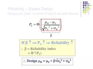
b. Design m R = m S + b s S 2 + s R 2. Reliability – Based Design. Observe for Case 1 in which R and S are both Normal. If b P S Reliability b = Reliability index = F -1 (P S ). What makes a structure safer?. Normally we cannot control loading

Reliability – Based Design
E N D
Presentation Transcript
b Design mR = mS + bsS2 + sR2 Reliability – Based Design Observe for Case 1 in which R and S are both Normal If b PS Reliability b = Reliability index = F-1(PS)
What makes a structure safer? • Normally we cannot control loading Building as ex, we can’t control wind • We can only control on resistance side We can build a larger column • Two ways: 1) higher μR higher mean capacity 2) lower σR better quality control to reduce variation of strength of a column How about correlation between failure modes, or loading?
Case 3: If R is discrete, S is continuous P(R = r) 0.6 0.3 0.1 r 5 6 7 Example on Case 3 S = N(5, 1)
P(R = r) 1 r 5 6 7 P(R = r) 1 .8 .6 .4 .2 r 6 5 7 Challenge 1 • What if R is not discrete? Example on Case 4 S = N(5, 1) Cut into strips trapezium
Challenge 1 • If we use 5 strips,
Central Limit Theorem S will approach a normal distribution regardless the individual probability distribution of Xiif N is large enough More importantly, S will have a mean of And Variance of Or a Variance of
fE(e) (a) E(E) = 0 1/2 -1 0 +1 e P4.27
(b) P(E < 0.01% of length of segment) (area under rectangular curve) (c) T = total mean = E1 + E2 +…+ E124 E(T) = 124 0 = 0 Var(T) = Var(E1) + Var(E2) +…+ Var(E124) = 124Var(E) = 124 1/3 = 41.33 sT = 6.43 Distribution of T Normal (C.L.T) \ P(T < 0.01% of 2 miles) Assume s.i. if not S.I., P ? By making more measurements, the % error is decreasing P(within given tolerance limit)
… X g(X) g’(mX) (X – mX) mx - mx Var(X) g(mX) mX X Taylor Series Approximation First order approximation:
If mK = 400 ; sK = 200 If M = 100 Example
K M M S.I. What if M is also random? mM = 100; sM = 20 then What if not S.I.?
Challenge 2 Product of many normal is log-normal? Transform Take log on both sides, and let S = ln P, X = ln Y with N (λ,ξ) And find μx, σx (This is “moments” of r.v. but we are NOT transforming to normal) By CLT, S is Normal with Then P can be calculated using the transformation formulae