Dynamic Branch Prediction
1. 2. 3. 4. 5. Dynamic Branch Prediction. Dynamic branch prediction schemes utilize run-time behavior of branches to make predictions. Usually information about outcomes of previous occurrences of branches are used to predict the outcome of the current branch.

Dynamic Branch Prediction
E N D
Presentation Transcript
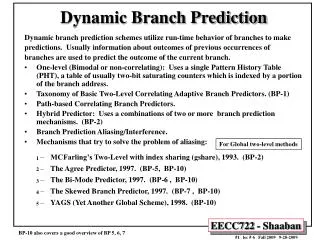
1 2 3 4 5 Dynamic Branch Prediction Dynamic branch prediction schemes utilize run-time behavior of branches to make predictions. Usually information about outcomes of previous occurrences of branches are used to predict the outcome of the current branch. • One-level (Bimodal or non-correlating): Uses a single Pattern History Table (PHT), a table of usually two-bit saturating counters which is indexed by a portion of the branch address. • Taxonomy of Basic Two-Level Correlating Adaptive Branch Predictors. (BP-1) • Path-based Correlating Branch Predictors. • Hybrid Predictor: Uses a combinations of two or more branch prediction mechanisms. (BP-2) • Branch Prediction Aliasing/Interference. • Mechanisms that try to solve the problem of aliasing: • MCFarling’s Two-Level with index sharing (gshare), 1993. (BP-2) • The Agree Predictor, 1997. (BP-5, BP-10) • The Bi-Mode Predictor, 1997. (BP-6 , BP-10) • The Skewed Branch Predictor, 1997. (BP-7 , BP-10) • YAGS (Yet Another Global Scheme), 1998. (BP-10) For Global two-level methods BP-10 also covers a good overview of BP 5, 6, 7
One-Level (Bimodal) Branch Predictors • One-level (bimodal or non-correlating) branch prediction uses only one level of branch history. • These mechanisms usually employ a table which is indexed by lower N bits of the branch address. • Each table entry (or predictor) consists of n history bits, which form an n-bit automaton or saturating counters. • Smith proposed such a scheme, known as the Smith Algorithm, that uses a table of two-bit saturating counters. (1985) • One rarely finds the use of more than 3 history bits in the literature. • Two variations of this mechanism: • Pattern History Table (PHT): Consists of directly mapped entries. • Branch History Table (BHT): Stores the branch address as a tag. It is associative and enables one to identify the branch instruction during IF by comparing the address of an instruction with the stored branch addresses in the table (similar to BTB). Pattern History Table (PHT) i.e Predictors From 551
One-Level Bimodal Branch Predictors Pattern History Table (PHT) Most common one-level implementation From 551 2-bit saturating counters (predictors) Sometimes referred to as Decode History Table (DHT) or Branch History Table (BHT) High bit determines branch prediction 0 = NT = Not Taken 1 = T = Taken N Low Bits of What if two or more branches have the same low N address bits? Table has 2N entries (also called predictors) . Not Taken (NT) 0 0 0 1 1 0 1 1 Example: For N =12 Table has 2N = 212 entries = 4096 = 4k entries Number of bits needed = 2 x 4k = 8k bits Taken (T) Update counter after branch is resolved: -Increment counter used if branch is taken - Decrement counter used if branch is not taken What if different branches map to the same predictor (counter)? This is called branch address aliasing and leads to interference with current branch prediction by other branches and may lower branch prediction accuracy for programs with aliasing.
One-Level Bimodal Branch Predictors Branch History Table (BHT) From 551 N Low Bits of 2-bit saturating counters (predictors) High bit determines branch prediction 0 = NT= Not Taken 1 = T = Taken 0 0 0 1 1 0 1 1 Not Taken (NT) Taken (T) Not a common one-level implementation (May lower impact of branch address aliasing (interference) on prediction performance)
Taken (T) 11 10 Not Taken (NT) 0 0 0 1 1 0 1 1 Taken (T) Taken (T) Taken (T) Not Taken (NT) Taken (NT) Predict Taken Predict Taken Predict Not Taken Predict Not Taken 00 01 Taken (T) 01 00 10 11 Not Taken (NT) Not Taken (NT) Not Taken (NT) Not Taken (NT) Basic Dynamic Two-Bit Branch Prediction: From 551 Two-bit Predictor State Transition Diagram (in textbook) Or Two-bit saturating counter predictor state transition diagram (Smith Algorithm): Not Taken (NT) Taken (T) The two-bit predictor used is updated after the branch is resolved
Prediction Accuracy of A 4096-Entry Basic One-Level Dynamic Two-Bit Branch Predictor N=12 2N = 4096 FP Misprediction Rate: Integer average 11% FP average 4% (Lower misprediction rate due to more loops) Integer Has, more branches involved in IF-Then-Else constructs the FP (potentially correlated branched) From 551
Correlating Branches Recent branches are possibly correlated: The behavior of recently executed branches affects prediction of current branch. Example: Branch B3 is correlated with branches B1, B2. If B1, B2 are both not taken, then B3 will be taken. Using only the behavior of one branch cannot detect this behavior. Occur in branches used to implement if-then-else constructs Which are usually more common in integer than floating point code Here aa = R1 bb = R2 DSUBUI R3, R1, #2 ; R3 = R1 - 2 BNEZ R3, L1 ; B1 (aa!=2) DADD R1, R0, R0 ; aa==0 L1: DSUBUI R3, R2, #2 ; R3 = R2 - 2 BNEZ R3, L2 ; B2 (bb!=2) DADD R2, R0, R0 ; bb==0 L2: DSUBUI R3, R1, R2 ; R3=aa-bb BEQZ R3, L3 ; B3 (aa==bb) B1 if (aa==2) aa=0; B2 if (bb==2) bb=0; B3 if (aa!==bb){ B1 not taken (not taken) B2 not taken (not taken) (not taken) B3 taken if aa=bb aa=bb=2 B3 in this case From 551
Two-Level Correlating Adaptive Predictors • Two-level correlating adaptive predictors were originally proposed by Yeh and Patt (1991). • They use two levels of branch history to account for the behavior of correlated branches in the supplied prediction. • The first level stored in a Branch History Register (BHR), or Table (BHT), usually one or more k-bit shift register(s). • The data in this register or table is used to index the second level of history, the Pattern History Table (PHT) or tables (PHTs) using an indexing function. • Yeh and Patt later (1993) identified nine variations (taxonomy) of this mechanism depending on how branch history in the first level and pattern history in the second level are kept: • Globally, • Per address, or • Per set (index bits). First Level: i.e more than one BHR Second Level: 1 2 3 BP-1
A General Two-level Branch Predictor (or Generic) Second Level: Or PHTs First Level: Register (BHR) or Table (BHT) or Path History Register (PHR) Last branch outcome k-bits • Examples of indexing functions: • Concatenate low address bits and BHR (GAp) • XOR low address bits and BHR (Gshare) Examples of other inputs: Per Address First Level: Low”a” bits of branch address (per address first level) Per Set First Level (with s=4 sets): i index bits of branch address used to divide branches into s = 2i sets e.g In paper #1 (BP-1) i=2 index bits 10, 11 used as branch set index to divide branches into s =4 sets and select between four BHRs in first level What if the indexing function for two or more branches map to the same predictor in the second level (this is called index aliasing)? Set index bits Branch address 11 10
Taxonomy of Two-level Adaptive Branch Prediction Mechanisms First Level First Level Second Level Adaptive Second Level Per Set First Level: i index bits of branch address used to divide branches into s = 2i sets e.g In paper #1 (BP-1) i=2 index bits 10, 11 used as branch set index to divide branches into s =4 sets and select between four BHRs in first level Per Address First Level: “a” low bits of branch address used to select from b = 2a BHT entries BP-1
Hardware Cost of Two-level Adaptive Prediction Mechanisms Storage requirements in bits • Neglecting logic cost, branch targets and assuming 2-bit (predictor) of pattern history for each PHT entry. The parameters are as follows: • k is the length of the history registers BHRs, • b is the number of BHT entries, and or number of PHTs in per address schemes • b = 2a where a is the number of low branch address used • s = 2i (i number of set index bits) is the number of sets of branches in first level (# of BHRs). • p = 2m (m number of set index bits) is the number of sets of branches in second level (# of PHTs). First Level { For per set schemes In First Level In Second Level (For both levels in bits) (PHTs) Each PHT has 2k entries (each 2 bit predictor) Thus each PHT requires 2x2k bits BP-1
Variations of global history Two-Level Adaptive Branch Prediction BP-1 First Level:Global, One BHR of size k bits, Second Level: One or more PHT(s) each of size = 2k predictors Here m =4 (16 second level sets) BHR BHR BHR First Level: Single BHR of size k bits One PHT b = 2a PPHTs p = 2m SPHTs GAx : Global schemes, first level is global, one BHR of size k bits
Correlating Two-Level Dynamic GAp Branch Predictors • Improve branch prediction by looking not only at the history of the branch in question but also at that of other branches using two levels of branch history. • Uses two levels of branch history: • First level (global): • Record the global pattern or history of the k most recently executed branches as taken or not taken. Usually a k-bit shift register. • Second level (per branch address): • b= 2a pattern history tables (PHTs) , each table entry has n bit saturating counter (usually n = 2 bits). • The low “a” bits of the branch address are used to select the proper branch prediction table (PHT) in the second level. • The k-bit global branch history register(BHR) from first level is used to select the correct prediction entry (predictor)within a the selected table, • Thus each of the b= 2a tables has 2k entries and each entry (predictor) is usually a 2-bit saturating counter. • Total number of bits needed for second level = 2a x 2 x 2k = b x 2 x 2k bits • In general, the notation: GAp (k,n) predictor means: • Record last k branches in first level BHR. • Each second level table (PHT) uses n-bit counters (each table entry has n bits). • Basic two-bit single-level Bimodal BHT is then a (0,2) predictor (k=0, no BHR). Last Branch 0 =Not taken 1 = Taken k-bit shift register Branch History Register (BHR) 1 One BHR BHR Pattern History Tables (PHTs) 2 predictor Size/Number of PHTs + k For first level BHR From 551
Organization of a Correlating Two-level GAp (2,2) Branch Predictor a= 4 Low 4 bits of address n= 2 k= 2 Global (1st level) One PHT Second Level Adaptive (16 PHTs) GAp High bit determines branch prediction 0 = Not Taken 1 = Taken 16 = 2a = 24 per address (2nd level) Selects correct PHT In this Example: a = # of low bits of branch address used = 4 Thus: b= 2a = 24 = 16 tables (PHTs) in second level k = # of branches tracked in first level (BHR) = 2 Thus: each table (PHT) in 2nd level has 2k = 22 = 4 entries (i.e each PHT size =4 predictors) n = # predictor size in PHTs = 2 Number of bits for 2nd level = 2a x 2 x 2k = 16 x 2 x 4 = 128 bits Selects correct entry (predictor) in selected PHT First Level Branch History Register (BHR) (2 bit shift register) (BHR) k = 2 From 551
Branch low-address bits used Branch low-address bits used a = 10 Size of BHR, k= 2 bits Prediction Accuracy of Two-Bit Dynamic Predictors Under SPEC89 a = 12 1024 PHTs each has 4 predictors Size of BHR, k= 2 bits Basic Basic Correlating Two-level Single (one) Level Gap (2, 2) FP Integer From 551
Branch Prediction Aliasing/Interference • Aliasing occurs when different branches point to (and use) the same prediction bits (predictor) this leads to interference with current branch prediction by other branches. • Address Aliasing:If the branch prediction mechanism is a one-level mechanism, lower bits of the branch address are used to index the table. Two branches with the same lower k bits point to the same prediction bits. • Index Aliasing:Occurs in two-level schemes when two or more branches have the same index into second level. • For example: In a PAg two-level scheme, the pattern history (second level) is indexed by the contents of history registers (BHRs). If two branches have the same k history bits (same BHR value or index) they will point to the same predictor entry in the global PHT. • Three different cases of aliasing/interference based on impact on prediction: • Constructive aliasing improves the prediction accuracy, • Destructive aliasing decreases the prediction accuracy, and • Harmless (or neutral) aliasing does not change the prediction accuracy. • An alternative classification of aliasing applies the "three-C" model of cache misses to aliasing/misprediction. Where aliasing is classified as three cases: • Compulsory aliasing/misprediction occurs when a branch substream is encountered for the first time. • Capacity aliasing/misprediction is due to the programs working set being too large to fit into the prediction data structures. Increasing the size of the data structures can reduce this effect. • Conflict aliasing/misprediction occurs when two concurrently-active branch substreams map to the same predictor-table entry. 1 2 3 1 2 3 Aliasing (address or Index) Interference
Index Aliasing/Interference in a Two-level Predictor • Index Aliasing occurs when different branches point to (and use) the same prediction bits (predictor): • - i.e two or more branches have the same index into second level. • This leads to interference with current branch prediction by other branches. Index Aliasing Example: Here branches A, B have the same index into second level Aliasing (address or index) Interference Chosen Predictor Aliased Index: Both branches A and B have the same index to level 2 i.e Interference (due to index aliasing) Index to second level PHT formed from branch address, branch history same index (aliasing) for two ore more branches BP-5
} FP (GAp) (GAs) (GAg) (GAp) } (GAs) Integer (GAg) Performance of Global history schemes with different branch history (BHR) lengths (k = 2-18 bits) • The average prediction accuracy of integer (int) and floating point (fp) programs by using global history schemes. These curves are cut of when the implementation cost exceeds 512K bits. Number of PHTs = b = 2a Where a is the number of low branch address or index bits used Size of each PHT = 2k Where k is the size of the BHR GAp fp GAp int GAs fp GAg int GAg fp GAs int For 9 SPEC89 benchmarks k (BHR) BP-1
} FP } Integer Performance of Global history schemes with different number of pattern history tables (1-1024 PHTs) Number of PHTs = b = 2a Where a is the number of low branch address or index bits used Size of each PHT = 2k Where k is the size of the BHR Number of PHTs = 2a Here “a” was varied from 0 to 10 210 = 1024 PHTs For 9 SPEC89 benchmarks GAg 1 PHT Log2 (1) =0 Or “a” These curves are cut of when the implementation cost exceeds 512K bits. BP-1
Number of bits needed (Size of BHR) Number of PHTs = b = 2a Where a is the number of low branch address or index bits used Size of each PHT = 2k Where k is the length of the BHR Most Cost-effective Global: 8K: GAs(7, 32) 128K: GAs (11, 32) 32 = 25 = Number of PHTs BP-1 For 9 SPEC89 benchmarks BHR length = k (here k= 7 or 11)
Notes On Global Schemes Performance • The performance of global history schemes is sensitive to branch history register (BHR) length. • Using one PHT (Gag) prediction accuracy is still rising with 18-bit BHR, improving 25% when BHR is increased from 2 to 18 bits. • Using 16 PHTs, prediction accuracy improved 10% when BHR is increased from 2 to 18 bits. • Lengthening the BHR increases the probability that the history the current branch needs is in the BHR and reduces pattern history (PHT) interference. • The performance of global history schemes is also sensitive to the number of pattern history tables (PHTs). • The pattern history of different branches interfere with each other if they map to the same PHT. • Adding more PHTs reduces the probability of pattern history interference by mapping interfering branches to different tables Why? Why? i.e. Global schemes suffer from a high level of index aliasing which results in excessive pattern history interference for short BHR length k and a small number of PHTs. Increasing BHR length and number of PHTs greatly reduces the level of index aliasing/pattern interference and thus improves prediction accuracy BP-1
BP-1 Variations of per-address historyTwo-Level Adaptive Branch Prediction First Level:Per Address, Branch History Table (BHT) with b=2a entries , each entry is a k-bit BHR Second Level: One or more PHT(s) each of size = 2k predictors Set Index bits Here m =4 (16 sets) One PHT BHT BHT BHT b = 2a PPHTs p = 2m SPHTs Size of BHT = b = 2a BHRs each k bits PAx : Per-Address schemes, first level is per-address, A BHT with 2a BHRs (each BHR of size or length k bits)
} (PAp) FP } (PAs) (PAg) Integer (PAp) (PAs) (PAg) Performance of Per-address history schemes with different branch history (BHR) lengths (k= 2-18 bits) Number of PHTs = b = 2a Where a is the number of low branch address or index bits used Size of each PHT = 2k Where k is the length of the BHR FP Better than Global schemes PAp fp PAp int PAg fp PAg int 9 SPEC89 benchmarks k (BHR) These curves are cut of when the implementation cost exceeds 512K bits. BP-1
} FP } Integer Performance of Per-address history schemes with different number of pattern history tables (1-1024 PHTs) Number of PHTs = b = 2a Where a is the number of low branch address or index bits used Size of each PHT = 2k Where k is the length of the BHR Number of PHTs = 2a Here “a” was varied from 0 to 10 FP Better than Global schemes k Integer worse than Global schemes 210 = 1024 PHTs PAg 1 PHT 9 SPEC89 benchmarks Or “a” PHTs These curves are cut of when the implementation cost exceeds 512K bits. BP-1
Number of bits needed 210 = 1024 PHTs Number of PHTs = b = 2a Where a is the number of low branch address or index bits used Size of each PHT = 2k Where k is the length of the BHR PHTs Most Cost-effective Per address: 8K: PAs(6, 16) 128K: PAs (8, 256) BP-1 BHR length = k (here k= 6 or 8) Number of PHTs Here (16 or 256)
Notes On Per-Address Schemes Performance • The prediction accuracy of per-address history schemes is not as sensitive to BHR length or number of PHTs as in global schemes • Using one PHT, integer prediction accuracy only improves 6% (compared to 25% for global) when BHR is increased from 2 to 18 bits. • Floating point performance is nearly flat when BHR length is larger than 6 bits. • Increasing number of PHTs results in a small performance improvement. • Average integer performance of global schemes is higher than per-address schemes: • Due to the large number of if-then-else statements in integer code which depend on the results of adjacent branches, therefore global schemes with better branch correlation perform better. • Average floating point performance of per-address schemes is higher than in global schemes: • Floating point programs contain more loop-control branches which exhibit periodic (non-correlated) branch behavior. • This periodic branch behavior is better retained in multiple BHRs, as a result performance is better in per-address history schemes. i.e. Per-address schemes suffer from a lower level of index aliasing (and thus less resulting pattern history interference) for short BHR length k and a small number of PHTs than in global schemes. Thus, performance improvement from increasing BHR length and number of PHTs is less than that exhibited in global schemes. Why? Why? BP-1
Variations of per-set history Two-Level Adaptive Branch Prediction BP-1 Set Index bits Here m =4 (16 sets) i First-Level Set Index Bits In paper PB-1 i = 2, thus 4 sets in first level (BHT with 4 BHRs) s = 2i BHRs s = 2i BHRs s = 2i BHRs p = 2m SPHTs b = 2a PPHTs Here i = 2 s = 22 = 4 sets in level 1 SAx : Per-Set schemes, first level is per-set, A BHT with s= 2i BHRs, s number of first-level branch sets (each BHR of size or length k bits)
} FP } Integer Performance of Per-set history schemes with different branch history (BHR) lengths (2-18 bits) First level: 4 sets or 4 BHRs (set index address bits 10-11, same block of 1K address) SAp fp (SAp) SAp int (SAs) SAs fp SAg fp (SAg) (SAp) SAs int (SAs) SAg int (SAg) k 9 SPEC89 benchmarks Number of PHTs = b = 2a Where a is the number of low branch addressor index bits used Size of each PHT = 2k Where k is the length of the BHR (BHR) These curves are cut of when the implementation cost exceeds 512K bits. BP-1
} FP } Integer Performance of Per-set history schemes with different number of pattern history tables (1-1024 PHTs) Number of PHTs = b = 2a Where a is the number of low branch addressor index bits used Size of each PHT = 2k Where k is the length of the BHR Number of PHTs = 2a Here “a” was varied from 0 to 10 210 = 1024 PHTs SAg 1 PHT 9 SPEC89 benchmarks Or “a” These curves are cut of when the implementation cost exceeds 512K bits. i=2 set index bits 10, 11 used as branch set index to divide branches into s =4 sets in first level (BHT has 4 BHRs) BP-1
Number of bits needed 210 = 1024 PHTs Most Cost-effective Per Set: 8K: SAs(6, 4x16) 128K: SAs (9, 4x32) BP-1 BHR length = k (here k= 6 or 9) Number of PHTs (here 4x16 or 4x32)
Notes On Per-Set Schemes Performance/Cost • Increasing the BHR length improves integer prediction accuracy significantly (similar to global schemes). • The performance of per-set schemes is less sensitive to the increase of number of PHTs than in global schemes but more sensitive than per-address schemes. • Floating point performance does not improve significantly when 4x16 or 4x256 PHTs are used. This is similar to per-address schemes. • This is due to partitioning the branches into sets (4 sets in this study using 4 BHTs) according to their addresses (index bits). Why? i.e. The level of index aliasing (and resulting pattern history interference) for a small number of PHTs is lower than in global schemes but higher than per-address schemes. Thus, performance improvement from increasing the numbe of PHTs is less than that exhibited in global schemes but more than per address schemes. BP-1
Comparison of the most effective configuration of each class of Two-Level Adaptive Branch Prediction with an implementation cost of 8K bits Global: GAs (7, 32) Per-address: PAs (6, 16) Per-set: SAs (6, 4x16) XAx (k, # of PHTs) BP-1
Comparison of the most effective configuration of each class of Two-Level Adaptive Branch Prediction with an implementation cost of 128K bits Global: GAs (11, 32) Per-address: PAs (8, 256) Per-set: SAs (9, 4x32) XAx (k, # of PHTs) BP-1
Performance Summary of Basic Two-level Branch Prediction Schemes • Global history schemes perform better than other schemes on integer programs but require higher implementation costs to be effective overall • Integer programs contain many if-then-else branches which are effectively predicted by global schemes due to their better correlation with other previous branches • However, global schemes require long BHR and or many PHTs to reduce interference for effective overall performance. • Per-Address history schemes perform better than other schemes on floating point programs and require lower implementation costs to be effective. • Floating point programs contain many frequently-executed loop-control branches with periodic behavior which is better retained with a per-address BHT. • Pattern history of different branches interfere less than in global schemes, hence fewer PHTs are needed. • Per-set schemes have integer performance similar to global schemes. They also have floating point performance similar to per-address schemes • To be effective, per-set schemes have even higher implementation costs due to the separate PHTs for each set (4 level 1 sets in this study). BP-1
Path-Based Prediction • Ravi Nair proposed (1995) to use the path leading to a conditional branch rather than the branch history in the first level to index the second level PHTs. • The global branch history register (BHR) of a GAp scheme is replaced by a Path History Register (PHR), which encodes the addresses of the targets of the preceding “p” branches. • The path history register could be organized as a “g” bit shift register which encodes q bits of the last p target addresses, where g = p x q. • The hardware cost of such a mechanism is similar to that of a GAp scheme. If b branches are kept in the prediction data structure the cost is: g + b x 2 x 2g • The performance of this mechanism is similar or better than a comparable branch history schemes for the case of no context switching (worse with context switching, longer warm-up time). • For the case that there is context switching, that is, if the processor switches between multiple processes running on the system, Nair proposes flushing the prediction data structures at regular intervals to improve accuracy. In such a scenario the mechanism performs slightly better than a comparable GAp predictor. Vs. GAp Where b = Number of PHTs = 2a A possible disadvantage of path-based prediction
A Path-based Prediction Mechanism p branch targets First Level: q bits each PHR Replaces BHR in GAp a bits g = p x q Second Level: b = 2a PHTs Each of size 2g Storage cost in bits for both levels (similar to Gap): g + 2a x 2 x 2g
Hybrid Predictors(Also known as tournament or combined predictors) BP-2 • Hybrid predictors are simply combinations of two (most common) or more branch prediction mechanisms. • This approach takes into account that different mechanisms may perform best for different branch scenarios. • McFarling presented (1993) a number of different combinations of two branch prediction mechanisms. • He proposed to use an additional 2-bit counter selector array which serves to select the appropriate predictor for each branch. • One predictor is chosen for the higher two counts, the second one for the lower two counts. The selector array counter used is updated as follows: • If the first predictor is wrong and the second one is right the selector counter used counter is decremented, • If the first one is right and the second one is wrong, the selector counter used is incremented. • No changes are carried out to selector counter used if both predictors are correct or wrong. e.g. global vs. per-address Predictor Selector Array Counter Update
A Generic Hybrid Predictor Branch Prediction Which branch predictor to choose Usually only two predictors are used (i.e. n =2) e.g. As in Alpha, IBM POWER 4, 5, 6 BP-2
11 10 01 00 Use P1 Use P2 X X BP-2 MCFarling’s Hybrid Predictor Structure The hybrid predictor contains an additional counter array (predictor selector array) with 2-bit up/down saturating counters. Which serves to select the best predictor to use. Each counter in the selector array keeps track of which predictor is more accurate for the branches that share that counter. Specifically, using the notation P1c and P2c to denote whether predictors P1 and P2 are correct respectively, the selector counter is incremented or decremented by P1c-P2c as shown. Both wrong P2 correct P1 correct Both correct Selector Counter Update Predictor Selector Array e.g Per-Address e.g Global Branch Address Here two predictors are combined (a Low Bits of Address) (Current example implementations: IBM POWER4, 5, 6)
MCFarling’s Hybrid Predictor Performance by Benchmark (Single Level) (global two-level) (Combined) BP-2
MCFarling’s Combined Predictor Performance by Size (GAp) One Level (Gap) BP-2
The Alpha 21264 Branch Prediction • The Alpha 21264 uses a two-level adaptive hybrid method combining two algorithms (a global history and a per-branch history scheme) and chooses the best according to the type of branch instruction encountered • The prediction table is associated with the lines of the instruction cache. An I-cache line contains 4 instructions along with a next line and a set predictor. • If an I-cache line is fetched that contains a branch the next line will be fetched according to the line and set predictor. For lines containing no branches or unpredicted branches the next line predictor point simply to the next sequential cache line. • This algorithm results in zero delay for correct predicted branches but wastes I-cache slots if the branch instruction is not in the last slot of the cache line or the target instruction is not in the first slot. • The misprediction penalty for the alpha is 11 cycles on average and not less than 7 cycles. • The resulting prediction accuracy is about 95% very good. • Supports up to 6 branches in flight and employs a 32-entry return address stack for subroutines.
Alpha 21264 Branch Prediction (BHR) Predictor Selector Array Gshare? Gag? Pag? BHT Per-address (Also similar to IBM POWER4, 5, 6)
Sample Processor Branch Prediction Comparison Processor ReleasedAccuracyPrediction Mechanism Cyrix 6x86 early '96 ca. 85% PHT associated with BTB Cyrix 6x86MX May '97 ca. 90% PHT associated with BTB AMD K5 mid '94 80% PHT associated with I-cache AMD K6 early '97 95% 2-level adaptive associated with BTIC and ALU Intel Pentium late '93 78% PHT associated with BTB Intel P6 mid '96 90% 2 level adaptive with BTB PowerPC750 mid '97 90% PHT associated with BTIC MC68060 mid '94 90% PHT associated with BTIC DEC Alpha early '97 95% Hybrid 2-level adaptive associated with I-cache HP PA8000 early '96 80% PHT associated with BTB SUN UltraSparc mid '95 88%int PHT associated with I-cache 94%FP S+D S+D S+D PHT = One Level S+D : Uses both static (ISA supported) and dynamic branch prediction
Interference Reduction in Global Prediction Schemes • Gshare, 1993. (BP-2) • The Filter Mechanism, 1996. (BP-3) • The Agree Predictor, 1997. (BP-5) • The Bi-Mode Predictor, 1997. (BP-6) • The Skewed Branch Predictor, 1997. (BP-7) • YAGS (Yet Another Global Scheme), 1998. (BP-10) 1 2 3 4 5 Not covered here BP-10 also covers a good overview of BP 5, 6, 7
1 BP-2 MCFarling's gshare Predictor gshare = global history with index sharing • McFarling noted (1993) that using global history information might be less efficient than simply using the address of the branch instruction, especially for small predictors. • He suggests using both global history (BHR) and branch address by hashing them together. He proposed using the XOR of global k-bit branch history register (BHR) and k low branch address bits to index into the second level PHT. • Since he expects that this indexing function to distribute pattern history states used more evenly among available predictors (in second level PHT) than just using the BHR as an index (GAg). • The result is that this mechanism reduces the level of index aliasing and resulting interference and thus outperforms conventional global schemes (e.g GAg, GAp). • This mechanism uses less hardware than GAp, since both branch history (first level) and pattern history (second level) are kept globally (similar to GAg). • The hardware cost for k history (BHR) bits is k + 2 x 2k bits, neglecting costs for logic (Cost similar to GAg). Index Function gshare is one one the most widely implemented two level dynamic branch prediction schemes
gshare Predictor Branch and pattern history are kept globally. History and branch address are XORed and the result is used to index the PHT. First Level BHR (k bits) k low bits of branch address XOR (bitwise XOR) Index Into Second Level 2-bit saturating counters (predictors) Second Level PHT One Pattern History Table (PHT) with 2k entries (predictors) Cost in bits = k + 2 x 2k (similar to Gag) BP-2
gshare Performance PAg GAg SPEC89 used BP-2
2 The Agree Predictor • The Agree Predictor is a scheme that tries to deal with the problem of aliasing in global schemes, proposed by Sprangle, Chappell, Alsup and Patt • They distinguish three approaches to counteract the interference problem: • Increasing predictor size to cause conflicting branches to map to different table locations. (i.e increase BHR bits k, and/or number of PHTs, 2a) • Selecting a history table indexing function (into second level) that distributes history states evenly among available counters (gshare does this). • Separating different classes of branches so that they do not use the same prediction scheme. • The Agree predictor converts negative interference into positive or neutral interference by attaching a biasing bit to each branch, for instance in the BTB or instruction cache, which predicts the most likely outcome of the branch. • In addition, the Agree predictor also offsets/improves global predictors bad loop performance. • The 2-bit counters of the branch prediction now predict whether or not the biasing bit is correct or not. The counters are updated after the branch has been resolved, agreement with the biasing bit leads to incrementing the counters, if there is no agreement the counter is decremented. • The biasing bit could be determined by the direction the branch takes at 1-the first occurrence, or 2- by the direction most often taken by the branch. in global schemes Possible such classes: branches with tendency to be taken or not taken i.e agree with bias bit Operation/ Update at runtime BP-5 BP-10